Einstein’s General Relativity

Derivations, Applications and Reflections – by Albert Prins

Part IV – Experiments and Verifications


4 Experiments Confirming Einstein’s Theory

In this chapter we discuss a series of experiments that empirically support Einstein’s general theory of relativity. A central tool in the analysis of these experiments is the Schwarzschild solution of the Einstein field equations.

The following experiments are discussed:

  • The Hafele–Keating experiment (see section 4.1)
  • The motion of particles in a gravitational field (see section 4.2)
  • The deflection of light near massive bodies (see section 4.3)
  • The precession of planetary perihelia, especially Mercury (see section 4.4)
  • The Shapiro time delay (see section 4.5)
  • The calculation of the trajectory of a projectile in a strong gravitational field (see section 4.8)

Together, these experiments provide strong evidence for the validity of general relativity. In each case, the Schwarzschild metric provides a mathematical framework that accurately explains the observed phenomena.

4.1 Experiment 1 – The Hafele & Keating Experiment Using the Schwarzschild Equation

Derivation based on: A Hafele & Keating-like thought experiment, by Paul B. Andersen, October 16, 2008 (Andersen, 2008).

The famous Hafele–Keating experiment tested quantitative predictions of relativity, particularly time dilation due to both motion (special relativity) and gravity (general relativity).

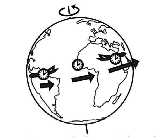
In this experiment, two airplanes equipped with cesium clocks were flown simultaneously around the Earth in opposite directions. A third cesium clock remained at a fixed location on Earth (in Washington). The results showed that the clocks onboard experienced different time dilation effects depending on their direction of motion and position relative to the Earth.

The clock on the eastward-flying aircraft moved along with the Earth’s rotation. As a result, it had a higher velocity relative to the non-rotating center of the Earth than the ground-based clock. This led to stronger time dilation: the clock lagged behind.

In contrast, the westward-flying aircraft moved against the Earth’s rotation, resulting in a lower velocity relative to the Earth’s center, and therefore weaker time dilation: this clock ran ahead. This difference in time progression shows that the passage of time depends on the observer’s motion — an effect already predicted by Einstein in 1905 in his original paper on special relativity.

vector_4_1
All three clocks move eastward. Even if the airplane flying westward relative to the air moves westward, the air itself moves eastward due to the Earth's rotation.
Source: (Crowell, March 11, 2018)

Objective and Setup

  • Objective: Direct experimental test of Einstein’s predictions for time dilation due to both motion (special relativity) and gravity (general relativity).
  • Setup: Cesium clocks were flown eastward and westward around the Earth, while a reference clock remained on Earth. The time differences between these clocks were measured and compared with theoretical predictions.

Theoretical Framework: Schwarzschild Metric

The Schwarzschild metric describes spacetime outside a spherically symmetric massive body such as the Earth:

\begin{align} c^2 d\tau^2=\left(1-\frac{2GM}{ c^2r}\right) c^2 dt^2-\left(1-\frac{2GM}{ c^2r} \right)^{-1} dr^2 -r^2 d\theta^2-r^2 \sin^2\theta \, d\phi^2 \label{eq:R00} \end{align}

Where:

  • t: coordinate time, measured by a hypothetical clock far from any gravitational field;
  • τ: proper time, measured by a clock moving with the observer at position r;
  • r: distance from the center of the Earth;
  • θ: polar angle relative to the North Pole;
  • : azimuthal angle relative to a fixed meridian;
  • G: gravitational constant;
  • M: mass of the Earth;
  • c: speed of light.

The Schwarzschild metric uses a universal (spherical) coordinate system with its origin at the Earth's center of mass. The Earth rotates within this coordinate system. Changes in the angles θ and describe motion over the Earth's surface.

Small changes in time and space are denoted by dt, dr, , and d∅. Note that dt represents the time change for a hypothetical observer far from gravitational influences; it is not directly measured time but a theoretical coordinate time.

The actual time measured by a clock at a given location is , the proper time.

We will use the Schwarzschild metric to derive an approximate formula describing the time dilation of the clocks based on their position and motion. We will then also present the full (exact) solution. Although the latter is more complex, it can be handled effectively using computational tools such as Excel and provides accurate results.

4.1.1 Approximate Formula for Time Dilation

We approximate the situation in which the clocks move along circular paths around the Earth: either at sea level or at some height above the Earth's surface. Since the paths are circular, we have dr = 0. Furthermore, we assume that the motion takes place in the equatorial plane, so that θ = π/2 is constant and therefore dθ = 0.

The Schwarzschild metric then simplifies to:

\begin{align} c^2 d\tau^2=\left(1 - \frac{2GM}{c^2 r}\right) c^2 dt^2-r^2 d\phi^2 \label{eq:R01} \end{align}

Dividing by \(c^2\) gives:

\begin{align} d\tau^2=\left(1 - \frac{2GM}{c^2 r}\right) dt^2-\frac{r^2}{c^2} \left(\frac{d\phi}{dt} \right)^2 dt^2 \label{eq:R02} \end{align}

Using the definition of orbital velocity \(v=r \frac{d\phi}{dt}\), we obtain:

\begin{align} d\tau=\sqrt{1 - \frac{2GM}{c^2 r} - \frac{v^2}{c^2}}\, dt \label{eq:R03} \end{align}

Since the terms \(\frac{2GM}{c^2r}\) and \(\frac{v^2}{c^2}\) are very small compared to 1, we apply a first-order Taylor approximation:

\begin{align} \sqrt{1-x}\approx 1-\tfrac{1}{2}x \quad \text{for }\, x\ll 1 \label{eq:R04} \end{align}

where \(x=\frac{2GM}{c^2r}+\frac{v^2}{c^2}\). This yields:

\begin{align} d\tau\approx\left(1-\frac{GM}{c^2 r}-\frac{v^2}{2c^2}\right)dt \label{eq:R05} \end{align}

Since \(r\) and \(v\) are constant, we can integrate directly:

\begin{align} \tau=\left(1-\frac{GM}{c^2 r}-\frac{v^2}{2c^2}\right) t+\tau_0 \label{eq:R06} \end{align}

We now compare two clocks. Clock 1 is located on the Earth's surface, with radius \(r_1\), the distance from the Earth's center, and velocity \(v_1\), due to Earth's rotation. For this clock:

\begin{align} d\tau_1=\left(1-\frac{GM}{c^2 r_1}-\frac{v_1^2}{2c^2}\right)dt \label{eq:R07} \end{align}

For clock 2, for example in an aircraft at altitude \(h\), with radius \(r_2\) and velocity \(v_2\), we have:

\begin{align} d\tau_2=\left(1-\frac{GM}{c^2 r_2}-\frac{v_2^2}{2c^2}\right)dt \label{eq:R08} \end{align}

The ratio between the two time intervals then becomes:

\begin{align} d\tau_2=\frac{1 - \frac{GM}{c^2 r_2} - \frac{v_2^2}{2c^2}}{1 - \frac{GM}{c^2 r_1} - \frac{v_1^2}{2c^2}}\, d\tau_1 \label{eq:R09} \end{align}

Using the approximation:

\begin{align} (1-\varepsilon)^{-1} \approx 1+\varepsilon, \label{eq:R10} \end{align}
we obtain:

\begin{align} d\tau_2 \approx \left( 1 - \frac{GM}{c^2 r_2} - \frac{v_2^2}{2c^2} \right) \left( 1 + \frac{GM}{c^2 r_1} + \frac{v_1^2}{2c^2} \right) d\tau_1 \label{eq:R11} \end{align}

\begin{align} d\tau_2 \approx \left[ 1 + \frac{GM}{c^2 r_1} + \frac{v_1^2}{2c^2} - \frac{GM}{c^2 r_2}\left( 1 + \frac{GM}{c^2 r_1} + \frac{v_1^2}{2c^2} \right) - \frac{v_2^2}{2c^2}\left( 1 + \frac{GM}{c^2 r_1} + \frac{v_1^2}{2c^2} \right) \right] d\tau_1 \label{eq:R12} \end{align}

Since the terms \(\frac{GM}{c^2 r_1}, \frac{v_1^2}{2c^2}, \frac{GM}{c^2 r_2}, \frac{v_2^2}{2c^2}\) are very small, their products can be neglected. This gives:

\begin{align} d\tau_2 \approx \left[ 1 + \frac{GM}{c^2 r_1}+\frac{v_1{}^2}{2c^2}-\frac{GM}{c^2 r_2}-\frac{v_2{}^2}{2c^2}\right] d\tau_1 \label{eq:R13} \end{align}

\begin{align} d\tau_2 \approx \left[ 1 + \frac{GM}{c^2}\left(\frac{1}{r_1}-\frac{1}{r_2}\right) + \frac{v_1^2 - v_2^2}{2c^2} \right] d\tau_1 \label{eq:R14} \end{align}

If we assume that both clocks start at \(\tau_1=\tau_2=0\), the integration is straightforward:

\begin{align} \tau_2 \approx \left[ 1 + \frac{GM}{c^2}\left(\frac{1}{r_1}-\frac{1}{r_2}\right) + \frac{v_1^2 - v_2^2}{2c^2} \right] \tau_1 \label{eq:R15} \end{align}

Comparison between clocks

For a clock on the Earth's surface \((r_1, v_1)\) and a clock in an aircraft \((r_2, v_2)\):

\begin{align} \tau_2 - \tau_1 \approx \left[ \frac{GM}{c^2}\left(\frac{1}{r_1}-\frac{1}{r_2}\right) + \frac{v_1^2 - v_2^2}{2c^2} \right]\tau_1 \label{eq:R16} \end{align}

Suppose clock 1 is located on the Earth's surface with radius \(R\), and clock 2 in an aircraft at altitude \(h\). Then \(r_2 = R + h\). Since \(h \ll R\), we can approximate:

\begin{align} \frac{1}{R} - \frac{1}{R+h} \approx \frac{h}{R^2} \quad\Rightarrow\quad \frac{GM}{c^2}\left(\frac{1}{R}-\frac{1}{R+h}\right) \approx \frac{gh}{c^2} \label{eq:R17} \end{align}

Thus:

\begin{align} \tau_2 - \tau_1 \approx \left[ \frac{GM}{c^2}\left(\frac{1}{R}-\frac{1}{R+h}\right) + \frac{v_1^2 - v_2^2}{2c^2} \right]\tau_1 \label{eq:R18} \end{align}
\begin{align} \approx \left[ \frac{GM}{c^2}\left(\frac{h}{R^2}\right) + \frac{v_1^2 - v_2^2}{2c^2} \right]\tau_1 \label{eq:R19} \end{align}

If we assume \(h/R \ll 1\) and \(g = GM/R^2\), then:

\begin{align} \tau_2 - \tau_1 = \left( \frac{gh}{c^2} - \frac{v_2^2 - v_1^2}{2c^2} \right)\tau_1 \label{eq:R20} \end{align}

Since \(v_1 = v_{\text{earth}}\) (Earth’s rotational velocity) and \(v_2 = v_{\text{plane}} + v_{\text{earth}}\), we obtain:

\begin{align} v_1^2 - v_2^2 = v_{\text{earth}}^2 - (v_{\text{plane}} + v_{\text{earth}})^2 = -v_{\text{plane}}^2 - 2 v_{\text{earth}} v_{\text{plane}} \label{eq:R21} \end{align}

Substituting into (\ref{eq:R20}) gives:

\begin{align} \tau_{\text{plane}} - \tau_{\text{earth}} = \left( \frac{gh}{c^2} - \frac{v_{\text{plane}}(v_{\text{plane}} + 2v_{\text{earth}})}{2c^2} \right)\tau_{\text{earth}} \label{eq:R22} \end{align}

This equation is fully derived from the Schwarzschild equation with several approximations. It agrees with the approximation used in the original Hafele–Keating experiment.

Remark 1. If the velocity of the aircraft is interpreted as ground speed, then at altitude \(h\) it can be approximated as:

\begin{align} v_2=\frac{R + h}{R}\left(v_{\text{plane}} + v_{\text{earth}}\right) \label{eq:R24} \end{align}

In that case, the above formula must be adjusted accordingly.

Remark 2. A more precise treatment of \(v_1\) and \(v_2\) follows in the next chapter, where the velocities are derived more specifically based on the chosen coordinate system.

4.1.2 Elaboration of v1 and v2 in Equation (\ref{eq:R20})

The velocity \(v_1\) in equation (\ref{eq:R20}) is the velocity of a stationary point on the equator of the Earth's surface. It is expressed as:

\begin{align} v_1 = r_1 \frac{d\phi}{dt} \label{eq:R24a} \end{align}

where dt is the coordinate time in the ‘universal’ reference frame. However, since measurements on the Earth's surface are performed with respect to the local proper time \(\tau\), a conversion is required.

Using the chain rule:

\begin{align} v_{1,t}= r_1 \frac{d\phi}{dt}= r_1 \frac{d\phi}{d\tau} \frac{d\tau}{dt}= v_{1,\tau} \frac{d\tau}{dt} \label{eq:R25} \end{align}

We now use the Schwarzschild metric (in the equatorial plane and with \(dr = 0\)) to determine \(\frac{d\tau}{dt}\):

\begin{align} c^2 d\tau^2=\left(1 - \frac{2GM}{c^2 r_1}\right)c^2 dt^2- r_1^2 \left(\frac{d\phi}{d\tau} \right)^2 d\tau^2 \label{eq:R26} \end{align}

After rearranging:

\begin{align} \left[1 + \frac{r_1^2}{c^2}\left(\frac{d\phi}{d\tau}\right)^2 \right] d\tau^2=\left(1 - \frac{2GM}{c^2 r_1}\right) dt^2 \label{eq:R27} \end{align}

We define:

\begin{align} \sigma^2 = 1 - \frac{2GM}{c^2 r} \label{eq:R28} \end{align}

Then:

\begin{align} \left(1 + \frac{v_{1,\tau}^2}{c^2}\right) d\tau^2= \sigma_1^2 dt^2 \label{eq:R29} \end{align}
\begin{align} \left(\frac{d\tau}{dt}\right)^2=\frac{\sigma_1^2}{1 + \frac{v_{1,\tau}^2}{c^2}} \label{eq:R30} \end{align}

Substitution into equation (26) gives:

\begin{align} v_{1,t}^2=v_{1,\tau}^2\left(\frac{d\tau}{dt}\right)^2=v_{1,\tau}^2\frac{\sigma_1^2}{1 + \frac{v_{1,\tau}^2}{c^2}} \label{eq:R31} \end{align}

This expression shows that \(\frac{d\tau}{dt}\), the conversion between coordinate time and proper time, depends on the rotational velocity of the Earth, \(v_{1,\tau}\), measured in local proper time.

Now consider an airplane flying eastward. The total velocity at ground level (measured in proper time) is:

\begin{align} v_{1\tau \text{_plane}}=v_{\text{plane_}\tau}+v_{1\tau \text{_earth}}=r_1 \frac{d\phi}{d\tau} \label{eq:R32} \end{align}

where:

  • \(v_{\text{plane_}\tau}\): velocity of the airplane relative to the Earth's surface
  • \(v_{1\tau \text{_earth}}\): rotational velocity of the Earth

Angular velocity in the universal frame

The corresponding angular velocity in the universal frame is:

\begin{align} r_1 \frac{d\phi}{dt} = r_1 \frac{d\phi}{d\tau}\frac{d\tau}{dt} = \left( v_{\text{plane_}\tau}+v_{1\tau \text{_earth}} \right) \frac{d\tau}{dt} \label{eq:R33} \end{align}

\begin{align} \frac{d\tau}{dt} = \frac{\sigma_1}{\sqrt{\left(1 + \frac{v_{1\tau\text{_earth}}^{2}}{c^{2}}\right)}} \label{eq:R34} \end{align}

\begin{align} \frac{d\phi}{dt} =\left( v_{\text{plane_}\tau}+v_{1\tau \text{_earth}} \right) \frac{\sigma_1}{r_1\sqrt{\left(1 + \frac{v_{1\tau\text{_earth}}^{2}}{c^{2}}\right)}} \label{eq:R35} \end{align}

Here we have calculated the rotational velocity (angular velocity) in the universal frame. This is valid at any level, i.e., any distance from the center. However, the velocity itself is given by r times this angular velocity.

Velocity at the level of the aircraft

\( v_{\text{plane},\tau} \) is the measured velocity of the aircraft at ground level and with respect to proper time, which is the only available time at that level. \( v_{\text{earth},\tau} \) is the rotational velocity of a stationary point on Earth with respect to the universal frame, but measured using proper time at ground level.

The velocity of the aircraft in the universal frame at altitude \( r_2 \) is:

\begin{align} v_{2t}=r_2 \frac{d\phi}{dt}=\frac{r_2}{r_1}\frac{\sigma_1}{\sqrt{1 + \frac{v_{1\tau \text{_earth}}^2}{c^2}}}\left( v_{\text{plane_}\tau}+v_{1\tau \text{_earth}} \right) \label{eq:R36} \end{align}

We split this velocity into an 'Earth rotation' and an 'aircraft' component:

\begin{align} v_{2t} = v_{2t\text{_earth}} + v_{2t\text{_plane}} \label{eq:R37} \end{align}

With:

\begin{align} v_{2t\text{_earth}} = \frac{r_2}{r_1}\, \frac{\sigma_1 v_{1\tau\text{_earth}}}{\sqrt{1 + \frac{v_{1\tau\text{_earth}}^2}{c^2}}} \label{eq:R38} \end{align}

And:

\begin{align} v_{2t\text{_plane}} = v_{2t} - v_{2t\text{_earth}} = \frac{r_2}{r_1}\, \frac{\sigma_1 v_{\text{plane_}\tau}}{\sqrt{1 + \frac{v_{1\tau\text{_earth}}^2}{c^2}}} \label{eq:R39} \end{align}

Summary of the result:

The conversion of velocity at ground level to the universal frame:

\begin{align} v_{1t\text{_earth}} = v_{1\tau\text{_earth}} \, \frac{\sigma_{\text{earth}}}{1 + \sqrt{\frac{v_{1\tau\text{_earth}})^2}{c^2}}} \label{eq:R40} \end{align}

The velocity \( v_2 \) of the aircraft in the universal frame is:

\begin{align} v_{2t} = \frac{r_2}{r_1}\, \frac{ \sigma_{\text{earth}}\left(v_{\text{plane_}\tau} + v_{\text{earth_}\tau}\right) }{ \sqrt{1 + \frac{v_{1\tau\text{_earth}}^2}{c^2}} } \label{eq:R41} \end{align}

Substitution into equation (\ref{eq:R20}):

\begin{align} \tau_2 - \tau_1 = \left( \frac{gh}{c^2} - \frac{v_2^2 - v_1^2}{2c^2} \right) \tau_1 \label{eq:R42} \end{align}

becomes:

\begin{align} \tau_2 - \tau_1 = \left( \frac{gh}{c^2} - \frac{ \sigma_{\text{earth}}^2 }{ 1 + \frac{(v_{1\tau\text{_earth}})^2}{c^2} } \cdot \frac{1}{2c^2} \left[ \left( \frac{R+h}{R} \right)^2 \left( v_{\tau\text{_plane}} + v_{\tau\text{_earth}} \right)^2 - v_{1\tau\text{_earth}}^2\right]\right) \;\tau_1 \label{eq:R43} \end{align}

This equation describes the time dilation between a clock on the Earth's surface and a clock aboard an aircraft, taking into account both gravitational and velocity-dependent effects, all based on locally measurable quantities.

4.1.3 The Exact Derivation

Instead of an approximation, we now perform an exact derivation, fully based on the Schwarzschild metric. We begin with equation (\ref{eq:R03}):

\begin{align} d\tau = \sqrt{\left(1 - \frac{2GM}{c^2 r} - \frac{v^2}{c^2}\right)} \, dt \label{eq:R44} \end{align}

Since \( r \) and \( v \) are constant, the integration is straightforward:

\begin{align} \tau = \sqrt{\left(1 - \frac{2GM}{c^2 r} - \frac{v^2}{c^2}\right)} \, t + \tau_0 \label{eq:R45} \end{align}

The goal is to compare the proper time of different clocks. As a reference, we take the clock on the Earth's surface. Other clocks are located in aircraft, at higher altitudes and with different velocities. Even the clock on Earth has a non-zero velocity due to Earth's rotation.

For the clock on the Earth's surface (radius \( r_1 \), velocity \( v_1 \)):

\begin{align} d\tau_1 = \sqrt{\left(1 - \frac{2GM}{c^2 r_1} - \frac{v_1^2}{c^2}\right)} \, dt \label{eq:R46} \end{align}

For the clock in the aircraft (radius \( r_2 \), velocity \( v_2 \)):

\begin{align} d\tau_2 = \sqrt{\left(1 - \frac{2GM}{c^2 r_2} - \frac{v_2^2}{c^2}\right)} \, dt \label{eq:R47} \end{align}

To find the ratio between the two proper times, we divide these expressions:

\begin{align} \frac{d\tau_2}{d\tau_1} =\sqrt{ \frac{ 1 - \frac{2GM}{c^2 r_2} - \frac{v_2^2}{c^2} }{ {1 - \frac{2GM}{c^2 r_1} - \frac{v_1^2}{c^2}} }} \label{eq:R48} \end{align}

With equal initial time \( \tau_2(0) = \tau_1(0) = 0 \), the solution is:

\begin{align} \tau_2 =\left(\sqrt{ \frac{ 1 - \frac{2GM}{c^2 r_2} - \frac{v_2^2}{c^2} }{ 1 - \frac{2GM}{c^2 r_1} - \frac{v_1^2}{c^2} }}\right) \tau_1 \label{eq:R49} \end{align}

Time difference between two clocks

\begin{align} \tau_2 - \tau_1 = \left(\sqrt{ \frac{ 1 - \frac{2GM}{c^2 r_2} - \frac{v_2^2}{c^2} }{ 1 - \frac{2GM}{c^2 r_1} - \frac{v_1^2}{c^2} }} - 1 \right) \tau_1 \label{eq:R50} \end{align}

Let \( r_1 = R \), the radius of the Earth, and \( r_2 = R + h \), the altitude of the aircraft, then this becomes:

\begin{align} \tau_2 - \tau_1 = \left(\sqrt{ \frac{ 1 - \frac{2GM}{c^2 (R+h)} - \frac{v_2^2}{c^2} }{ 1 - \frac{2GM}{c^2 R} - \frac{v_1^2}{c^2} }} - 1 \right) \tau_1 \label{eq:R51} \end{align}

Velocities and gravitational effects

In this expression:

  • \( v_1 \) is the rotational velocity of a point on the Earth's surface (eastward direction),
  • \( v_2 \) is the velocity of the aircraft relative to the universal reference frame.

Both velocities are derived later in equations (\ref{eq:R70}) and (\ref{eq:R71}) of chapter 4.1.5.

\begin{align} \tau_{\text{plane}} - \tau_{\text{earth}} = \left(\sqrt{ \frac{ 1 - \frac{2GM}{c^2 (R+h)} - \frac{v_2^2}{c^2} }{ 1 - \frac{2GM}{c^2 R} - \frac{v_1^2}{c^2} }} - 1 \right) \tau_{\text{earth}} \label{eq:R52} \end{align}

Using the Schwarzschild radius \( R_s = \frac{2GM}{c^2} \), we rewrite this as:

\begin{align} \tau_{\text{plane}} - \tau_{\text{earth}} = \left(\sqrt{ \frac{ 1 - \frac{R_s}{R+h} - \frac{v_2^2}{c^2} }{ 1 - \frac{R_s}{R} - \frac{v_1^2}{c^2} }} - 1 \right) \tau_{\text{earth}} \label{eq:R53} \end{align}

Conclusion

This equation is an exact expression, directly derived from the Schwarzschild metric. It shows how the difference in proper time between a clock on Earth and a clock in an aircraft is influenced by:

  • Gravitational time dilation: clocks at higher altitude (weaker gravity) run faster.
  • Kinematic time dilation: clocks moving faster run slower.

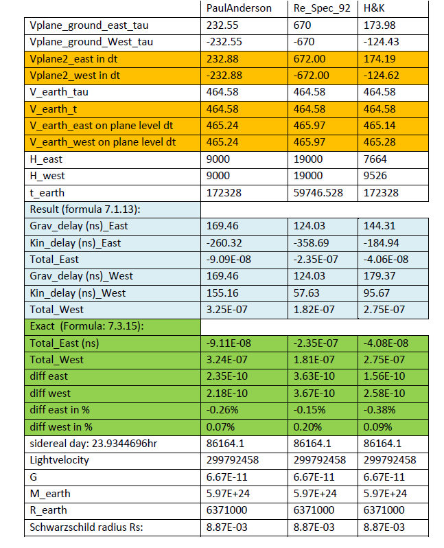
Calculations based on the performed experiments:

vector_4_1_3_1

Conclusion

The approximations are accurate within a precision of 0.4%.

Practical Application

  • Earth’s rotational velocity (equator): \( v_{\text{earth}} \) is approximately 464.58 m/s (based on the sidereal day).
  • Aircraft: velocity relative to the Earth's surface, corrected for altitude.
  • Altitude effect: \( h \) is typically a few kilometers, \( R \) (Earth) approximately \( 6.371 \times 10^{6}\,\text{m} \).

Results and Interpretation

  • Eastward flying clock: higher velocity relative to the Earth's center → stronger kinematic time dilation → clock runs slower.
  • Westward flying clock: lower velocity relative to the Earth's center → weaker time dilation → clock runs faster.
  • Gravitational effect: clocks at higher altitude (aircraft) run faster due to weaker gravity.

Experimental Outcome

  • The measured time differences matched exactly with the predictions of general relativity, with an accuracy of less than 0.4%.
  • Both the approximate and exact formulas (derived from the Schwarzschild metric) are consistent with observations.

Summary

  • The Hafele–Keating experiment is a direct, quantitative confirmation of Einstein’s theory of relativity.
  • The Schwarzschild metric provides the mathematical framework for explaining these time dilation effects.
  • Both effects — motion and gravity — are essential and are measured and explained simultaneously.

4.1.4 The velocity of a stationary point on the equator at the Earth's surface

To calculate the velocity of a stationary point on the equator, we must first determine the Earth's rotation period: the sidereal day.

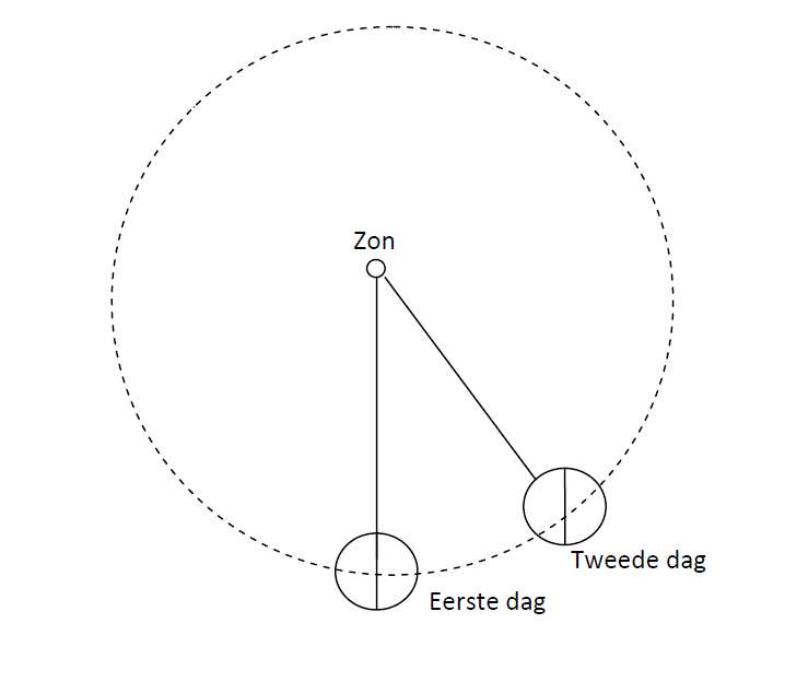
Sidereal day versus solar day

A normal day (24 hours) is the time between two successive highest positions of the Sun in the sky. This time is based on the solar cycle, not on the Earth's actual rotation.

Due to the Earth's annual orbit around the Sun, the Earth makes one extra rotation per year relative to the fixed stars. In one year (365.25 solar days), the Earth therefore rotates 366.25 times about its axis relative to the stars.

From this follows the duration of one sidereal day:

\begin{align} T_{\text{sidereal}}=\frac{365{,}25}{366{,}25}\cdot24\cdot3600=86164{,}1\ \text{s} \label{eq:R54} \end{align}

Converted to hours:

\begin{align} \frac{86164{,}1}{3600}=23{,}93447\ \text{hours} \label{eq:R55} \end{align}

That is: 23 hours, 56 minutes, and 4 seconds.

vector_4_1_4

Velocity at the equator

With the Earth's radius

\begin{align} R = 6371 \ \text{km}=6{,}371 \times 10^{6} \ \text{m}, \label{eq:R56} \end{align}

we can calculate the circumference at the equator:

\begin{align} \text{Circumference}=2\pi R=2\pi \times 6{,}371 \times 10^{6}\approx4{,}003 \times 10^{7}\ \text{m}. \label{eq:R57} \end{align}

The velocity of a stationary point on the equator (relative to a non-rotating reference frame) is then:

\begin{align} v_{\text{earth}}=\frac{2\pi R}{T_{\text{sidereal}}}=\frac{4{,}003 \times 10^{7}}{86164{,}1}=464{,}58\ \text{m/s}. \label{eq:R58} \end{align}

For comparison: if we incorrectly used a 24-hour day, we would obtain:

\begin{align} v=\frac{2\pi R}{86400}=463{,}3\ \text{m/s}. \label{eq:R59} \end{align}

Summary

  • A sidereal day lasts approximately 23 hours, 56 minutes, and 4 seconds.
  • The velocity of a stationary point on the equator is approximately 464.58 m/s.
  • The difference between a sidereal day and a solar day leads to a measurable difference in velocity, which is important for relativistic calculations, such as in the Hafele–Keating experiment.

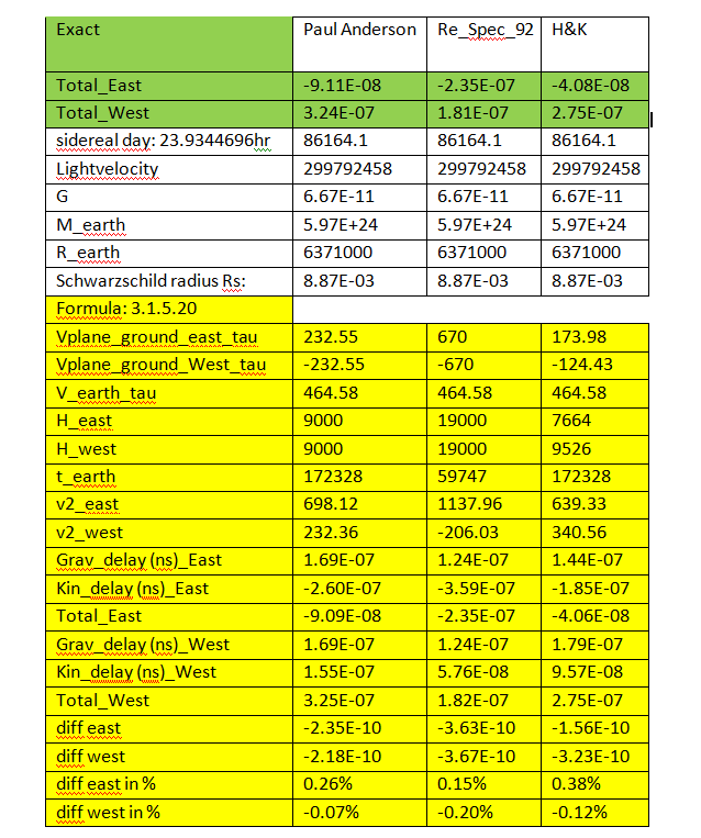
4.1.5 Correction to the derivation based on Paul Anderson

In Anderson's original derivation, the velocity of the aircraft is introduced relative to the Earth's surface. However, in his formula (\ref{eq:R02}), this velocity is expressed with respect to the coordinate time \(dt\), while clocks in motion measure proper time \(d\tau\). This requires a correction: the velocity of the object must be expressed relative to its own clock, i.e., via \(d\tau\).

Starting point: The full Schwarzschild relation

We take as our starting point equation (\ref{eq:R01}) from chapter 4.1.1, without approximation:

\begin{align} c^{2}\,d\tau^{2} = \left(1 - \frac{2GM}{c^{2}r}\right)c^{2}\,dt^{2} - r^{2}\,d\phi^{2} \label{eq:R60} \end{align}

Dividing by \(c^{2}\) gives:

\begin{align} d\tau^{2} = \left(1 - \frac{2GM}{c^{2}r}\right)dt^{2} - \frac{r^{2}}{c^{2}}\left(\frac{d\phi}{d\tau}\right)^{2}d\tau^{2} \label{eq:R61} \end{align}

We rewrite this as:

\begin{align} d\tau^{2} \left(1 + \frac{r^{2}}{c^{2}}\left(\frac{d\phi}{d\tau}\right)^{2}\right)= \left(1 - \frac{2GM}{c^{2}r}\right)dt^{2} \label{eq:R62} \end{align}

And thus:

\begin{align} d\tau = \sqrt{ \frac{1 - \dfrac{2GM}{c^{2}r}} {1 + \dfrac{r^{2}}{c^{2}}\left( \dfrac{d\phi}{d\tau}\right)^{2}} }\,dt \label{eq:R63} \end{align}

With:

\begin{align} v_{\tau} = r\,\frac{d\phi}{d\tau} \label{eq:R64} \end{align}

Thus:

\begin{align} d\tau_{1} = \sqrt{ \frac{1 - \dfrac{2GM}{c^{2}r_{1}}}{1 + \dfrac{v_{1}^{2}}{c^{2}}}}\,dt \label{eq:R65} \end{align}
\begin{align} d\tau_{2} =\sqrt{ \frac{1 - \dfrac{2GM}{c^{2}r_{2}}} {1 + \dfrac{v_{2}^{2}}{c^{2}}}}\,dt \label{eq:R66} \end{align}

We then write:

\begin{align} d\tau_{2}=\sqrt{\frac{1 - \dfrac{2GM}{c^{2}r_{2}}}{1 + \dfrac{v_{2}^{2}}{c^{2}}}}\sqrt{ \frac{1 + \dfrac{v_{1}^{2}}{c^{2}}}{1 - \dfrac{2GM}{c^{2}r_{1}}}}\,d\tau_{1} \label{eq:R67} \end{align}

This yields the relation between both proper times:

\begin{align} \tau_{2}=\sqrt{\frac{1 - \dfrac{2GM}{c^{2}r_{2}}}{1 + \dfrac{v_{2}^{2}}{c^{2}}}}\sqrt{ \frac{1 + \dfrac{v_{1}^{2}}{c^{2}}}{1 - \dfrac{2GM}{c^{2}r_{1}}}}\,\tau_{1} \label{eq:R68} \end{align}

If we take \(\tau_{1} = \tau_{\text{earth}}\) (clock at sea level) and \(\tau_{2} = \tau_{\text{plane}}\), we obtain:

\begin{align} \tau_{\text{plane}} - \tau_{\text{earth}} =\left[\sqrt{\frac{1 - \dfrac{2GM}{c^{2}r_{2}}}{1 + \dfrac{v_{2}^{2}}{c^{2}}}}\sqrt{\frac{1 + \dfrac{v_{1}^{2}}{c^{2}}}{1 - \dfrac{2GM}{c^{2}r_{1}}}}- 1\right]\tau_{\text{earth}} \label{eq:R69} \end{align}

Here \(r_{1} = R\), the radius of the Earth. The distance of the clock in an aircraft is then \(R + h\). This gives:

\begin{align} \tau_{\text{plane}} - \tau_{\text{earth}}=\left[\sqrt{\frac{\left(1 - \dfrac{2GM}{c^{2}(R + h)} \right)\left( 1 + \dfrac{v_{\text{earth}}^{2}}{c^{2}} \right)} {\left( 1 - \dfrac{2GM}{c^{2}R} \right)\left(1 + \dfrac{v_{2}^{2}}{c^{2}}\right)}}- 1\right]\tau_{\text{earth}} \label{eq:R70} \end{align}

Or using the Schwarzschild radius \(R_{s} = \dfrac{2GM}{c^{2}}\):

\begin{align} \tau_{\text{plane}} - \tau_{\text{earth}}=\left[\sqrt{\frac{\left(1 - \dfrac{R_s}{(R + h)} \right)\left( 1 + \dfrac{v_{\text{earth}}^{2}}{c^{2}} \right)} {\left( 1 - \dfrac{R_s}{R} \right)\left(1 + \dfrac{v_{2}^{2}}{c^{2}}\right)}}- 1\right]\tau_{\text{earth}} \label{eq:R71} \end{align}

Relative velocity at flight altitude

The ground speed of the aircraft (relative to the Earth's surface) must be converted to a coordinate-independent velocity at flight altitude:

\begin{align} v_{2}=\left(v_{\text{earth}} + v_{\text{plane (relative to earth point)}}\right)\cdot \frac{R + h}{R} \label{eq:R72} \end{align}

Up to this point, the formula is without approximations.

After applying first-order Taylor approximations to equation (\ref{eq:R70}), as done earlier, the result becomes:

\begin{align} \tau_{\text{plane}} - \tau_{\text{earth}}=\left(\left[1 - \frac{GM}{c^{2}(R + h)}\right]\left[1 + \frac{GM}{c^{2}R}\right]\left[1 + \frac{v_{\text{earth}}^{2}}{2c^{2}}\right]\left[1 - \frac{v_{2}^{2}}{2c^{2}}\right]- 1\right)\tau_{\text{earth}} \label{eq:R73} \end{align}

This can be rewritten as:

\begin{align} \tau_{\text{plane}} - \tau_{\text{earth}}=\left(\left[1 + \frac{GM}{c^{2}}\left(\frac{1}{R} - \frac{1}{R + h}\right)\right]\left[1 + \frac{v_{\text{earth}}^{2} - v_{2}^{2}}{2c^{2}} \right]- 1\right)\tau_{\text{earth}} \label{eq:R74} \end{align}
\begin{align} \tau_{\text{plane}} - \tau_{\text{earth}}=\left(\left[1 + \frac{GM}{c^{2}}\frac{h}{R^{2}}\right] \left[1 + \frac{v_{\text{earth}}^{2} - v_{2}^{2}}{2c^{2}}\right]- 1\right)\tau_{\text{earth}} \label{eq:R75} \end{align}
\begin{align} \tau_{\text{plane}} - \tau_{\text{earth}}=\left(\frac{GM}{c^{2}}\frac{h}{R^{2}}+ \frac{v_{\text{earth}}^{2} - v_{2}^{2}}{2c^{2}}\right)\tau_{\text{earth}} \label{eq:R76} \end{align}

With \(g = \dfrac{GM}{R^{2}}\), this becomes:

\begin{align} \tau_{\text{plane}} - \tau_{\text{earth}}=\left(\frac{gh}{c^{2}}- \frac{v_{2}^{2} - v_{\text{earth}}^{2}}{2c^{2}}\right)\tau_{\text{earth}} \label{eq:R77} \end{align}

Note on velocities and reference frames

The velocity of the aircraft is given as ground speed. It is not immediately clear whether this is measured relative to the clock on Earth or the clock in the aircraft. Let us assume that the Earth-based clock is intended. In that case, we must convert to the level of the aircraft, which means considering the clock at that level. We do this via the time \(t\) in the universal frame.

If we consider \(\dfrac{d\phi_{\text{earth}}}{dt}\), this represents the Earth's rotational velocity in the universal frame. We can find the Earth's velocity at sea level by multiplying \(\dfrac{d\phi_{\text{earth}}}{dt}\) by \(R\), the distance from the center. The Earth's velocity as seen from the aircraft level is \((R + h) \dfrac{d\phi_{\text{earth}}}{dt}\). The same applies to the aircraft: at sea level, the relative aircraft velocity is \(R\dfrac{d\phi_{\text{plane}}}{dt}\), and at aircraft level \((R + h)\dfrac{d\phi_{\text{plane}}}{dt}\).

We now need to determine \(\dfrac{d\phi_{\text{earth}}}{dt}\) and \(\dfrac{d\phi_{\text{plane}}}{dt}\). We use from chapter 4.1.5 equation (4c):

\begin{align} v_{\tau} = r\,\frac{d\phi}{d\tau}= r\,\frac{d\phi}{dt}\,\frac{dt}{d\tau}\;\Rightarrow\; \frac{d\phi}{dt}= \frac{v_{\tau}}{r}\,\frac{d\tau}{dt} \label{eq:R78} \end{align}

Next, we use from chapter 4.1.5 equation (64):

\begin{align} \frac{d\tau}{dt}=\sqrt{\frac{1 - \dfrac{2GM}{c^{2}r}}{1 + \dfrac{v_{\tau}^{2}}{c^{2}}}} \label{eq:R79} \end{align}

Thus:

\begin{align} \frac{d\phi}{dt} =\frac{v_{\tau}}{r}\frac{d\tau}{dt}=\frac{v_{\tau}}{r}\sqrt{\frac{1 - \dfrac{2GM}{c^{2}r}}{1 + \dfrac{v_{\tau}^{2}}{c^{2}}}} \label{eq:R80} \end{align}

All components on the right-hand side are known.

At sea level:

\begin{align} \frac{d\phi_{\text{earth}}}{dt}=\frac{v_{\text{earth}}}{R}\sqrt{\frac{1 - \dfrac{2GM}{c^{2}R}}{1 + \dfrac{v_{\text{earth}}^{2}}{c^{2}}}} \label{eq:R81} \end{align}

And for the aircraft analogously:

\begin{align} \frac{d\phi_{\text{plane}}}{dt}=\frac{v_{\text{plane}}}{R}\sqrt{\frac{1 - \dfrac{2GM}{c^{2}R}} {1 + \dfrac{v_{\text{earth}}^{2}}{c^{2}}}} \label{eq:R82} \end{align}

Now at aircraft level:

\begin{align} v_{2}=v_{2\tau\text{_earth}} + v_{2\tau\text{_plane}}=(R + h)\left(\frac{d\phi_{ \text{earth}}}{dt}+ \frac{d\phi_{\text{plane}}}{dt}\right) \label{eq:R83} \end{align}

Thus:

\begin{align} v_{2} = \frac{R+h}{R} \sqrt{ \frac{1 - \dfrac{2GM}{c^{2}R}} {1 + \dfrac{v_{\text{earth}}^{2}}{c^{2}}} } \left( v_{\text{earth}} + v_{\text{plane}} \right) \label{eq:R84} \end{align}

Up to this point, \(v_{2}\) is still exact. With a first-order Taylor approximation:

\begin{align} v_{2}=\frac{R + h}{R}\sqrt{\left( 1 - \frac{GM}{c^{2}R}\right)\left(1 - \frac{v_{\text{earth}}^{2}}{2c^{2}} \right)}\left(v_{\text{earth}} + v_{\text{plane}}\right) \label{eq:R85} \end{align}

Thus, the relevant formula is:

\begin{align} v_{2}\approx\frac{R + h}{R}\left(1 - \frac{GM}{c^{2}R}- \frac{v_{\text{earth}}^{2}}{2c^{2}}\right) \left( v_{\text{earth}} + v_{\text{plane}}\right) \label{eq:R86} \end{align}

Result after Taylor approximation

Applied to equation (\ref{eq:R70}), this leads after linearization to:

\begin{align} \tau_{\text{plane}} - \tau_{\text{earth}}=\left(\frac{gh}{c^{2}}- \frac{v_{2}^{2} - v_{\text{earth}}^{2}}{2c^{2}}\right)\tau_{\text{earth}} \label{eq:R87} \end{align}

Conclusion

This revised approach corrects the inconsistency in the original derivation: velocities must be related to proper time, not coordinate time. After correction and Taylor approximation, the numerical deviation from the approximation in the previous chapter is less than \(0.4\%\), within the desired accuracy.

vector_4_1_5

4.1.6 Considerations regarding the Hafele–Keating experiment and the Schwarzschild metric

We begin with the general Schwarzschild equation:

\begin{align} ds^2 = c^2 d\tau^2 = \left(1 - \frac{2GM}{c^2 r}\right)c^2 dt^2 - \left(1 - \frac{2GM}{c^2 r}\right)^{-1} dr^2 - r^2 d\theta^2 - r^2 \sin^2\theta\, d\phi^2 \label{eq:R88} \end{align}

As used previously, we define:

\begin{align} \sigma =\sqrt{ 1 - \frac{2GM}{c^2 r}} \label{eq:R89} \end{align}

With this notation, equation (\ref{eq:R88}) is rewritten as:

\begin{align} ds^2 = c^2 d\tau^2 = \sigma^2 c^2 dt^2 - \sigma^{-2} dr^2 - r^2 d\theta^2 - r^2 \sin^2\theta\, d\phi^2 \label{eq:R90} \end{align}

In the Hafele–Keating experiment, the time of the clock of the United States Naval Observatory (USNO) and the velocity of an aircraft are measured. The question is: what do time and velocity represent in the context of the Schwarzschild metric?

There is a stationary clock at sea level on the equator, and two aircraft moving in the equatorial plane — one eastward, the other westward. Both aircraft follow circular paths with constant speed relative to the Earth's surface, but in opposite directions.

Since the experiment takes place in the equatorial plane, we assume that \(\theta = \pi/2\) is constant, and that \(r\) is also constant due to the circular motion. The Schwarzschild metric then simplifies to:

\begin{align} c^2 d\tau^2 = \left(1 - \frac{2GM}{c^2 r}\right)c^2 dt^2 - r^2 d\phi^2 \label{eq:R91} \end{align}

The coordinates \(t, r, \theta, \phi\) in the Schwarzschild metric can be interpreted as belonging to a universal (inertial) reference frame in which the Earth rotates. The clocks on the Earth's surface and in the aircraft are each in their own local inertial frames; their measured time is represented as proper time \(\tau\).

The universal coordinate time \(t\) is not directly measurable, but is a theoretical quantity. From equation (\ref{eq:R91}), it follows:

\begin{align} dt^2 = \frac{d\tau^2 + \frac{r^2}{c^2} d\phi^2}{1 - \frac{2GM}{c^2 r}} = \sigma^{-2}\left(d\tau^2 + \frac{r^2}{c^2} d\phi^2\right) \\ \notag = \sigma^{-2}\left(1 + \frac{r^2}{c^2}\left(\frac{d\phi}{d\tau}\right)^2\right)d\tau^2 \label{eq:R92} \end{align}

Assuming \(t = 0\) when \(\tau = 0\), this leads to:

\begin{align} t =\sigma^{-1}\sqrt{1 + \frac{r^2}{c^2}\left(\frac{d\phi}{d\tau}\right)^2}\,\tau= \sigma^{-1}\sqrt{1 + \frac{v^2}{c^2}}\,\tau \label{eq:R93} \end{align}

where \(v = r\, d\phi/d\tau\) is the velocity relative to the universal frame.

For velocities much smaller than \(c\), we can apply a first-order Taylor approximation:

\begin{align} t = \sigma^{-1}\sqrt{1 + \frac{v^2}{c^2}}\,\tau = \frac{1}{\sigma\sqrt{1 - \frac{v^2}{c^2}}}\,\tau = \frac{\gamma}{\sigma}\, \tau \label{eq:R94} \end{align}

with

\begin{align} \gamma =\frac{1}{ \sqrt{1 - \frac{v^2}{c^2}}} \label{eq:R95} \end{align}
the Lorentz factor.

This equation expresses how the proper time \(\tau\) of a moving clock relates to the coordinate time \(t\) in the Schwarzschild frame.

4.2 Experiment 2 – Motion of Particles in Schwarzschild Geometry

The derivations in this chapter are based on:

  • (Biesel, 2008) The Precession of Mercury’s Perihelion, Owen Biesel
  • (Magnan) Christian Magnan: Complete calculations of the perihelion precession of Mercury and the deflection of light by the Sun in General Relativity
  • (Pe’er, 2014) Asaf Pe’er: Schwarzschild Solution and Black Holes

We derive equations for the motion of particles in Schwarzschild geometry, as a basis for:

  • The precession of Mercury’s perihelion,
  • The deflection of light by the Sun,
  • The Shapiro experiment,
  • The calculation of a projectile trajectory.

We use the Schwarzschild metric as the starting point. Due to the symmetry in both the time coordinate \( t \) and the angular coordinate \( \phi \) (no metric component depends on these coordinates), Noether’s theorem applies: every continuous symmetry corresponds to a conservation law. This yields conservation of energy and conservation of angular momentum.

Overview of symbols used in §4.2
Symbol Meaning
\( v \) Total velocity with respect to coordinate time \( t \)
\( v_r = \dfrac{dr}{d\tau} \) Radial velocity (along the \( r \)-direction)
\( v_t = r\,\dfrac{d\phi}{d\tau} \) Transverse velocity (perpendicular to the \( r \)-direction)
\( \lambda \) Affine parameter (equal to proper time \( \tau \) for massive particles)
\( E \) Conserved energy per unit mass along the geodesic
\( L \) Conserved angular momentum per unit mass along the geodesic
\( \varepsilon \) \( 1 \) for massive particles, \( 0 \) for photons

Schwarzschild metric

The metric reads:

\begin{align} ds^2 = \sigma^2 c^2 dt^2 - \frac{dr^2}{\sigma^2} -\frac{r^2}{R^2_p} dR^2_p\,\theta^2 - \frac{r^2}{R^2_p} \sin^2\theta\, dR^2_p\,\phi^2 \label{eq:R96} \end{align}

To obtain the correct dimensions (all coordinates in meters), we set Rp=1m, making the coefficients dimensionless. This leads to the more common form:

\begin{align} ds^2 = \sigma^2 c^2 dt^2 - \frac{dr^2}{\sigma^2} - r^2 d\theta^2 - r^2 \sin^2\theta\, d\phi^2 \label{eq:R97} \end{align}

with:

\begin{align} \sigma =\sqrt{ 1 - \frac{2GM}{c^2 r}} =\sqrt{ 1 - \frac{R_s}{r}}, \qquad R_s = \frac{2GM}{c^2} \label{eq:R98} \end{align}

Metric coefficients

\begin{align} g_{00} = \sigma^2,\quad g_{11} = -\frac{1}{\sigma^2},\quad g_{22} = -r^2,\quad g_{33} = -r^2 \sin^2\theta \label{eq:R99} \end{align}

Contravariant components:

\begin{align} g^{00} = \frac{1}{\sigma^2},\quad g^{11} = -\sigma^2,\quad g^{22} = -\frac{1}{r^2},\quad g^{33} = -\frac{1}{r^2 \sin^2\theta} \label{eq:R100} \end{align}

Furthermore:

\begin{align} \frac{d\sigma}{dr} = \frac{R_s}{2 r^2 \sigma} \label{eq:R101} \end{align}

Derivatives of metric components

For the Schwarzschild metric with \(\sigma =\sqrt{ 1 - \dfrac{R_s}{r}}\) we find the following derivatives:

\begin{align} \frac{\partial g_{00}}{\partial r} = \frac{R_s}{r^2}, \qquad \frac{\partial g_{11}}{\partial r} = \frac{R_s}{r^2 \sigma^4}, \qquad \frac{\partial g_{22}}{\partial r} = -2r, \label{eq:R102} \end{align}

\begin{align} \frac{\partial g_{33}}{\partial r} = -2r \sin^2\theta, \qquad \frac{\partial g_{33}}{\partial \theta} = -2 r^2 \sin\theta \cos\theta. \label{eq:R103} \end{align}

Christoffel symbols

The Christoffel symbols are defined as:

\begin{align} \Gamma^\rho_{\mu\nu} = \frac{1}{2} g^{\rho\alpha} \left( \frac{\partial g_{\nu\alpha}}{\partial x^\mu} + \frac{\partial g_{\mu\alpha}}{\partial x^\nu} - \frac{\partial g_{\mu\nu}}{\partial x^\alpha} \right) \label{eq:R104} \end{align}

Some relevant non-zero symbols are:

\begin{align} \Gamma^{0}_{10} = \Gamma^{0}_{01} = \frac{1}{2} g^{00} \left(\frac{\partial g_{00}}{\partial r}\right) = \frac{R_s}{2 r^2 \sigma^2}, \label{eq:R105} \end{align}

\begin{align} \Gamma^{1}_{00} = \frac{1}{2} g^{11} \left(-\frac{\partial g_{00}}{\partial r}\right) = \frac{R_s}{2 r^2}\sigma^2, \qquad \Gamma^{1}_{11} = \frac{1}{2} g^{11} \left(\frac{\partial g_{11}}{\partial r}\right) = -\frac{R_s}{2 r^2 \sigma^2}, \label{eq:R106} \end{align}

\begin{align} \Gamma^{1}_{22} =\frac{1}{2} g^{11} \left(\frac{-\partial g_{22}}{\partial r}\right) = -r \sigma^2, \qquad \Gamma^{1}_{33} =\frac{1}{2} g^{11} \left(-\frac{\partial g_{33}}{\partial r}\right) = -r \sigma^2 \sin^2\theta, \label{eq:R107} \end{align}

\begin{align} \Gamma^{2}_{12} = \Gamma^{2}_{21} =\frac{1}{2} g^{22} \left(\frac{\partial g_{22}}{\partial r}\right) = \frac{1}{r}, \qquad \Gamma^{2}_{33} =\frac{1}{2} g^{22} \left(-\frac{\partial g_{33}}{\partial \theta}\right) = -\sin\theta\cos\theta, \label{eq:R108} \end{align}

\begin{align} \Gamma^{3}_{13} = \Gamma^{3}_{31} =\frac{1}{2} g^{33} \left(\frac{\partial g_{33}}{\partial r}\right) = \frac{1}{r}, \qquad \Gamma^{3}_{23} = \Gamma^{3}_{32} =\frac{1}{2} g^{33} \left(-\frac{\partial g_{33}}{\partial \theta}\right) = \cot\theta. \label{eq:R109} \end{align}

All other Christoffel symbols are zero.

Geodesic equations

We consider a geodesic worldline, which describes the natural trajectory of a particle in the absence of non-gravitational forces. The general geodesic equation reads:

\begin{align} \frac{d^2 x^\alpha}{d\lambda^2} + \Gamma^\alpha_{\mu\nu} \frac{dx^\mu}{d\lambda} \frac{dx^\nu}{d\lambda} = 0 \label{eq:R110} \end{align}

Geodesic equations per coordinate

We work out the four coordinates, where \( \lambda \) is the affine parameter (which here can be identified with proper time \( \tau \)):

For \( t \):

\begin{align} \frac{d^2 t}{d\lambda^2} + \Gamma^{t}_{\mu\nu} \frac{dx^\mu}{d\lambda} \frac{dx^\nu}{d\lambda} = \frac{d^2 t}{d\lambda^2} + 2\,\Gamma^{0}_{10} \frac{dt}{d\lambda} \frac{dr}{d\lambda} = \frac{d^2 t}{d\lambda^2} + 2\,\frac{R_s}{2 r^2 \sigma^2} \frac{dt}{d\lambda} \frac{dr}{d\lambda} = 0 \label{eq:R111} \end{align}

For \( r \):

\begin{align} \frac{d^2 r}{d\lambda^2} + \Gamma^{1}_{00}\left(\frac{dt}{d\lambda}\right)^2 + \Gamma^{1}_{11}\left(\frac{dr}{d\lambda}\right)^2 + \Gamma^{1}_{22}\left(\frac{d\theta}{d\lambda}\right)^2 + \Gamma^{1}_{33}\left(\frac{d\phi}{d\lambda}\right)^2 \label{eq:R112} \end{align}

\begin{align} =\frac{d^2 r}{d\lambda^2} + \sigma^2 \frac{R_s}{2 r^2} \left(\frac{dt}{d\lambda}\right)^2 - \frac{R_s}{2 r^2 \sigma^2} \left(\frac{dr}{d\lambda}\right)^2 - r\sigma^2 \left(\frac{d\theta}{d\lambda}\right)^2 - r\sigma^2 \sin^2\theta \left(\frac{d\phi}{d\lambda}\right)^2 = 0 \label{eq:R113} \end{align}

For \( \theta \):

\begin{align} \frac{d^2\theta}{d\lambda^2} + 2\,\Gamma^{2}_{12} \frac{dr}{d\lambda} \frac{d\theta}{d\lambda} + \Gamma^{2}_{33} \left(\frac{d\phi}{d\lambda}\right)^2 \label{eq:R114} \end{align}

\begin{align} =\frac{d^2\theta}{d\lambda^2} + 2\frac{1}{r} \frac{dr}{d\lambda} \frac{d\theta}{d\lambda} - \cos\theta\sin\theta \left(\frac{d\phi}{d\lambda}\right)^2 = 0 \label{eq:R115} \end{align}

For \( \phi \):

\begin{align} \frac{d^2\phi}{d\lambda^2} + 2\,\Gamma^{3}_{13} \frac{dr}{d\lambda} \frac{d\phi}{d\lambda} + 2\,\Gamma^{3}_{23} \frac{d\theta}{d\lambda} \frac{d\phi}{d\lambda} \label{eq:R116} \end{align}

\begin{align} =\frac{d^2\phi}{d\lambda^2} + 2\frac{1}{r} \frac{dr}{d\lambda} \frac{d\phi}{d\lambda} + 2\cos\theta\sin\theta \frac{d\theta}{d\lambda} \frac{d\phi}{d\lambda} = 0 \label{eq:R117} \end{align}

Summarized, these four component equations lead to:

\begin{align} \frac{d^2 t}{d\lambda^2} + 2\frac{R_s}{2 r^2 \sigma^2} \frac{dt}{d\lambda} \frac{dr}{d\lambda} = 0 \label{eq:R118} \end{align}

\begin{align} \frac{d^2 r}{d\lambda^2} + \sigma^2 \frac{R_s}{2 r^2} \left(\frac{dt}{d\lambda}\right)^2 - \frac{R_s}{2 r^2 \sigma^2} \left(\frac{dr}{d\lambda}\right)^2 - r\sigma^2 \left(\frac{d\theta}{d\lambda}\right)^2 - r\sigma^2 \sin^2\theta \left(\frac{d\phi}{d\lambda}\right)^2 = 0 \label{eq:R119} \end{align}

\begin{align} \frac{d^2\theta}{d\lambda^2} + 2\frac{1}{r} \frac{dr}{d\lambda} \frac{d\theta}{d\lambda} - \cos\theta\sin\theta \left(\frac{d\phi}{d\lambda}\right)^2 = 0 \label{eq:R120} \end{align}

\begin{align} \frac{d^2\phi}{d\lambda^2} + 2\frac{1}{r} \frac{dr}{d\lambda} \frac{d\phi}{d\lambda} + 2\cos\theta\sin\theta \frac{d\theta}{d\lambda} \frac{d\phi}{d\lambda} = 0 \label{eq:R121} \end{align}


Elegant approach according to Asaf Pe’er

We first follow the elegant approach of Asaf Pe’er from his article “Schwarzschild Solution and Black Holes” (Pe’er, 2014), after which we present a simpler approach.

According to Asaf Pe’er:

"At first sight, there seems little hope of solving this set of four coupled equations easily. Fortunately, our task is greatly simplified by the high degree of symmetry of the Schwarzschild metric."
— Asaf Pe'er, Schwarzschild Solution and Black Holes (2014)

Schwarzschild spacetime has four Killing fields: three due to spherical symmetry, and one due to time translation. Each Killing field leads, via Noether’s theorem, to a constant of motion for a free particle.

If \( K_\mu \) is a Killing field, then:

\begin{align} K_\mu \frac{dx^\mu}{d\lambda} = \text{constant} \label{eq:R122} \end{align}

Additionally, there is another constant of motion arising from metric compatibility. Along a geodesic worldline:

\begin{align} ds^2 = g_{\mu\nu} dx^\mu dx^\nu, \qquad \left(\frac{ds}{d\lambda}\right)^2 = c^2 \left(\frac{d\tau}{d\lambda}\right)^2 = c^2 \varepsilon = g_{\mu\nu} \frac{dx^\mu}{d\lambda} \frac{dx^\nu}{d\lambda} \label{eq:R123} \end{align}

Here:

  • \( \varepsilon = 1 \) for massive particles,
  • \( \varepsilon = 0 \) for photons (massless),
  • \( \varepsilon = -1 \) for spacelike geodesics.

Use of symmetries and conservation laws

Instead of directly solving the four coupled geodesic equations, we make use of symmetries that lead to conservation laws via Killing fields.

In flat spacetime, symmetries (via Noether) lead to familiar conserved quantities:

  • Time translation invariance → conservation of energy,
  • Rotational invariance → conservation of angular momentum.

Analogously, for the Schwarzschild metric:

  • Motion in a plane: Angular momentum preserves its direction → the particle moves in a plane. By coordinate rotation we may choose this as the equatorial plane:
    \begin{align} \theta = \frac{\pi}{2} \label{eq:R124} \end{align}
  • Conservation of energy: The timelike Killing field is:
    \begin{align} K^\mu = (1,0,0,0)_T \label{eq:R125} \end{align}
    The associated covariant component is:
    \begin{align} K_\mu = g_{\mu\nu} K^\nu = \left(1 - \frac{2GM}{c^2 r},\, 0,\, 0,\, 0\right) \label{eq:R126} \end{align}
    From this follows:
    \begin{align} K_\mu \frac{dx^\mu}{d\lambda} = \left(1 - \frac{2GM}{c^2 r}\right)\frac{dt}{d\lambda} = \frac{E}{c^2} \label{eq:R127} \end{align}
    or defined as:
    \begin{align} k = \left(1 - \frac{2GM}{c^2 r}\right)\frac{dt}{d\lambda} = \frac{E}{c^2} \label{eq:R128} \end{align}
  • Conservation of angular momentum: The Killing vector for rotations in \( \phi \) is:
    \begin{align} L^\mu = (0,0,0,-1)_T \label{eq:R129} \end{align}
    The covariant component is:
    \begin{align} L_\mu = g_{\mu\nu} L^\nu = (0,0,0,-r^2 \sin^2\theta) \label{eq:R130} \end{align}
    At \( \theta = \pi/2 \), we have \( \sin\theta = 1 \), so:
    \begin{align} r^2 \frac{d\phi}{d\lambda} = L \label{eq:R131} \end{align}

This yields the conserved quantities:

  • \( E \): energy per unit mass,
  • \( L \): angular momentum per unit mass.

For photons, these correspond to energy and angular momentum themselves. (more on angular momentum, see Appendix 10.)

Note that equation (\ref{eq:R131}) is the relativistic equivalent of Kepler’s second law: equal areas are swept out in equal times.


Alternative derivation

Although Asaf Pe’er notes that solving the full set of coupled geodesic equations appears complex, it turns out that some of these equations can be solved relatively easily. We demonstrate this using equations (\ref{eq:R118}) and (\ref{eq:R121}).

Step 1 — Using equation (\ref{eq:R118})

\begin{align} \frac{d^2 t}{d\lambda^2} + 2\,\frac{R_s}{2 r^2 \sigma^2} \frac{dt}{d\lambda} \frac{dr}{d\lambda} = 0 \label{eq:R132} \end{align}

where:

\begin{align} \sigma^2 =1 - \frac{2GM}{c^2r}= 1 - \frac{R_s}{r} \label{eq:R133} \end{align}

We multiply both sides by \( \sigma^2 \):

\begin{align} \sigma^2 \frac{d^2 t}{d\lambda^2} + \frac{R_s}{r^2} \frac{dt}{d\lambda} \frac{dr}{d\lambda} = 0. \label{eq:R134} \end{align}

Since \( \sigma^2 = 1 - \frac{R_s}{r} \), we rewrite:

\begin{align} \left(1 - \frac{R_s}{r}\right)\frac{d^2 t}{d\lambda^2} + \frac{R_s}{r^2} \frac{dt}{d\lambda} \frac{dr}{d\lambda} = 0. \label{eq:R135} \end{align}

We rewrite this:

\begin{align} \frac{d^2 t}{d\lambda^2} + \frac{R_s}{r^2} \frac{dt}{d\lambda} \frac{dr}{d\lambda} - \frac{R_s}{r} \frac{d^2 t}{d\lambda^2} = 0 \label{eq:R136} \end{align}

Or:

\begin{align} \frac{d}{d\lambda} \left( \frac{dt}{d\lambda} - \frac{R_s}{r}\frac{dt}{d\lambda} \right) = 0 \label{eq:R137} \end{align}

Thus:

\begin{align} \frac{d}{d\lambda} \left[ \frac{dt}{d\lambda}\left(1 - \frac{R_s}{r}\right) \right] = 0 \label{eq:R138} \end{align}

This shows that the expression

\begin{align} \frac{dt}{d\lambda}\left(1 - \frac{R_s}{r}\right) \label{eq:R139} \end{align}
is constant along the worldline.

We recognize this as the conserved quantity related to the total energy per unit mass of the particle. Multiplying by \( c \) gives:

\begin{align} \frac{cdt}{d\lambda}\left(1 - \frac{R_s}{r}\right) = \text{constant} = \frac{E}{c}\, \left(\text{total energy}\right) \label{eq:R140} \end{align}

Step 2 — Using equation (\ref{eq:R118})

We now proceed with equation (\ref{eq:R118}). To simplify the derivation, we assume motion in the equatorial plane:

\begin{align} \theta = \frac{\pi}{2}. \label{eq:R141} \end{align}

Then equation (\ref{eq:R118}) becomes:

\begin{align} \frac{d^2 \Phi}{d\lambda^2} + \frac{2}{r} \frac{dr}{d\lambda} \frac{d\Phi}{d\lambda} + 2\frac{\cos\theta}{ \sin\theta}\, \frac{d\theta}{d\lambda} \frac{d\Phi}{d\lambda} = 0. \label{eq:R142} \end{align}

Since in the equatorial plane

\begin{align} \theta = \frac{\pi}{2} \quad\Rightarrow\quad \cos\theta = 0,\;\; \sin\theta = 1, \label{eq:R143} \end{align}
the last term vanishes, leaving:

\begin{align} \frac{d^2 \Phi}{d\lambda^2} + \frac{2}{r} \frac{dr}{d\lambda} \frac{d\Phi}{d\lambda} = 0. \label{eq:R144} \end{align}

This leads to:

\begin{align} \frac{1}{r^2}\frac{d}{d\lambda}\left(r^2 \frac{d\phi}{d\lambda}\right)=0 \label{eq:R145} \end{align}

Which means that:

\begin{align} r^2\frac{d\phi}{d\lambda} \label{eq:R146} \end{align}

is constant along the geodesic worldline. This constant is recognized as the angular momentum per unit mass:

\begin{align} r^2\frac{d\phi}{d\lambda}=constant=L\left(angular\ momentum\right) \label{eq:R147} \end{align}

Summary of conserved quantities

Due to the symmetries, there are two conserved quantities:

  • Energy per unit mass:
    \begin{align} \left(1 - \frac{R_s}{r}\right)\frac{dt}{d\lambda} = \frac{E}{c^2} \label{eq:R148} \end{align}
  • Angular momentum per unit mass:
    \begin{align} L = r^2\,\frac{d\Phi}{d\lambda} \label{eq:R149} \end{align}

4.2.1 The Gravitational Potential

Using the previously derived conservation laws, we can now further analyze the motion of particles in the Schwarzschild metric. We begin by writing out equation (\ref{eq:R123}), using the conserved quantities from equations (\ref{eq:R140}) and (\ref{eq:R147}):

\begin{align} \left( 1 - \frac{2GM}{c^{2} r} \right) c^{2} \left( \frac{dt}{d\lambda} \right)^{2} - \left( 1 - \frac{2GM}{c^{2} r} \right)^{-1} \left( \frac{dr}{d\lambda} \right)^{2} - r^{2} \left( \frac{d\phi}{d\lambda} \right)^{2} = c^{2} \varepsilon \label{eq:R150} \end{align}

Substituting the conserved quantities E and L gives:

\begin{align} \left( 1 - \frac{2GM}{c^{2} r} \right) c^{2} \left( \frac{dt}{d\lambda} \right)^{2} - \left( 1 - \frac{2GM}{c^{2} r} \right)^{-1} \left( \frac{dr}{d\lambda} \right)^{2} - \frac{L^{2}}{r^{2}} = c^{2} \varepsilon \label{eq:R151} \end{align}

Multiplying this equation by \( 1 - \frac{2GM}{c^{2} r} \) and using \( \frac{E}{c} = c \frac{dt}{d\lambda} \left( 1 - \frac{2GM}{c^{2} r} \right) \) and \( L = r^{2} \frac{d\phi}{d\lambda} \), we rewrite:

\begin{align} \left( 1 - \frac{2GM}{c^{2} r} \right)^{2} c^{2} \left( \frac{dt}{d\lambda} \right)^{2} - \left( \frac{dr}{d\lambda} \right)^{2} - \left( 1 - \frac{2GM}{c^{2} r} \right) \frac{L^{2}}{r^{2}} + c^{2} \varepsilon = 0 \label{eq:R152} \end{align}

Substituting the expression for E yields:

\begin{align} \frac{E^{2}}{c^{2}} - \left( \frac{dr}{d\lambda} \right)^{2} - \left( 1 - \frac{2GM}{c^{2} r} \right) \frac{L^{2}}{r^{2}} + c^{2} \varepsilon = 0 \label{eq:R153} \end{align}

We have thus reduced the four coupled geodesic equations to a single differential equation for \( r(\lambda) \), which represents a major simplification.

We rewrite equation (\ref{eq:R20}) in the form:

\begin{align} \frac{1}{2} \left( \frac{dr}{d\lambda} \right)^{2} + V(r) = \frac{1}{2} \frac{E^{2}}{c^{2}} \label{eq:R154} \end{align}

with the effective potential \( V(r) \) defined as:

\begin{align} V(r) = \frac{1}{2} c^{2} \varepsilon - \frac{\varepsilon GM}{r} + \frac{L^{2}}{2 r^{2}} - \frac{GM L^{2}}{c^{2} r^{3}} \label{eq:R155} \end{align}

Equation (\ref{eq:R154}) is formally identical to the classical equation for the motion of a particle (with unit mass) in a one-dimensional potential \( V(r) \), where the total “energy” \( \frac{1}{2} \frac{E^{2}}{c^{2}} \) appears. Of course, the actual energy is \( E \), but this form makes the equation analogous to classical mechanics.

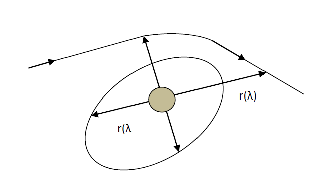
If we analyze the potential \( V(r) \) in equation (\ref{eq:R155}), we see that it differs from the Newtonian potential in only one respect: the last term. This term, proportional to \( 1/r^{3} \), represents a purely relativistic correction and plays an important role for small \( r \).

The terms can be interpreted as follows:

  • The first term is constant (rest energy for massive particles), depending on \( \varepsilon = 1 \) for massive particles and \( \varepsilon = 0 \) for photons;
  • The second term is the Newtonian gravitational potential;
  • The third term is the classical angular momentum potential;
  • The fourth term is the relativistic correction.

Note: despite the formal resemblance to classical mechanics, this does not describe the motion of a particle freely moving in one dimension. 
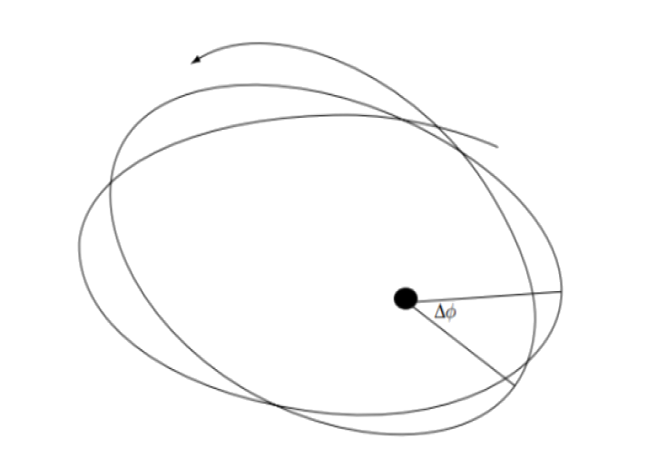
In reality, this concerns a particle moving in orbit around a massive object. The relevant quantities are not only \( r(\lambda) \), but also \( t(\lambda) \) and \( \phi(\lambda) \), which together describe the full spacetime trajectory.

vector_4_2_1
Figure 1 - Particle trajectories in a gravitational potential.

4.2.2 Intermezzo on Energy in Schwarzschild Geometry

In this intermezzo, we analyze the form of the energy as derived in equation (\ref{eq:R140}) from chapter 4.2. This energy is a conserved quantity in Schwarzschild geometry.

We begin with the relation:

\begin{align} \left( 1 - \frac{2GM}{c^{2} r} \right) \frac{dt}{d\lambda} = \frac{E}{m c^{2}} = \sigma^{2} \frac{dt}{d\lambda} \label{eq:R156} \end{align}

From which follows:

\begin{align} E = \sigma^{2} m c^{2} \frac{dt}{d\lambda} \label{eq:R157} \end{align}

The Schwarzschild metric reads:

\begin{align} ds^{2} = c^{2} d\tau^{2} = \sigma^{2} c^{2} dt^{2} - \frac{dr^{2}}{\sigma^{2}} - r^{2} d\theta^{2} - r^{2} \sin^{2}\theta \, d\phi^{2} \label{eq:R158} \end{align}

We use an affine parameter \( \lambda \) with \( d\tau = d\lambda \) and restrict ourselves to the equatorial plane \( \theta = \frac{\pi}{2} \).

\begin{align} \sigma^{2} c^{2} \left( \frac{dt}{d\lambda} \right)^{2} - \sigma^{-2} \left( \frac{dr}{d\lambda} \right)^{2} - r^{2} \left( \frac{d\phi}{d\lambda} \right)^{2} = c^{2} \varepsilon \label{eq:R159} \end{align}

Rewriting in terms of velocities with respect to coordinate time \( t \), we obtain:

\begin{align} \sigma^{2} c^{2} \left(\frac{dt}{d\lambda}\right)^{2} \;-\; \sigma^{-2} \left(\frac{dr}{dt}\right)^{2} \left(\frac{dt}{d\lambda}\right)^{2} \;-\; r^{2} \left(\frac{d\Phi}{dt}\right)^{2} \left(\frac{dt}{d\lambda}\right)^{2} = c^{2}\,\varepsilon \label{eq:R160} \end{align}

For massive particles, \( \varepsilon = 1 \):

\begin{align} \sigma^{2} \left( \frac{dt}{d\lambda} \right)^{2} \left( 1 - \frac{\sigma^{-2} \left( \frac{dr}{dt} \right)^{2} + r^{2} \left( \frac{d\phi}{dt} \right)^{2}}{\sigma^{2} c^{2}} \right) =\varepsilon= 1 \label{eq:R161} \end{align}
\begin{align} \left( \frac{dt}{d\lambda} \right)^{2}\left( 1 - \frac{v^2}{\sigma^2c^2}\right) =\frac{1}{\sigma^2} \label{eq:R162} \end{align}

which yields:

\begin{align} \frac{dt}{d\lambda} = \frac{1}{\sigma} \frac{1}{\sqrt{1 - \frac{v^{2}}{\sigma^{2} c^{2}}}} \label{eq:R163} \end{align}

Where \( v^{2} = \sigma^{-2} \left( \frac{dr}{dt} \right)^{2} + r^{2} \left( \frac{d\phi}{dt} \right)^{2} \)(\ref{eq:R66}) with the energy (equation (\ref{eq:R140})) leads to:

\begin{align} E = \sigma^{2} m c^{2} \frac{dt}{d\lambda} = \frac{\sigma m c^{2}} {\sqrt{1 - \frac{v^{2}}{\sigma^{2} c^{2}}} } = \gamma_\sigma \sigma m c^{2} \label{eq:R164} \end{align}

This conserved energy consists of:

  • Rest energy: \( E_{0} = \sigma m c^{2} \)
  • Relativistic kinetic energy:
    \begin{align} E_{\text{kin}} = \sigma m c^{2} \left( \frac{1}{\sqrt{1 - \frac{v^{2}}{\sigma^{2} c^{2}}}} - 1 \right) \label{eq:R165} \end{align}

In the non-relativistic limit \( v \ll c \), and using a first-order Taylor expansion of the square root, we obtain the “kinetic” energy:

\begin{align} E_{\text{kin}} \approx \sigma m c^{2} \left( 1+\frac{v^{2}}{2\sigma^{2}c^2}-1 \right)= \frac{m v^{2}}{2 \sigma} \label{eq:R166} \end{align}

4.2.2.1 Alternative approach via the metric

Start with the Schwarzschild equation:

\begin{align} ds^2 = c^2 d\tau^2 = \sigma^2 c^2 dt^2 - \sigma^{-2} dr^2 - r^2 d\theta^2 - r^2 \sin^2\theta\, d\phi^2 \label{eq:R167} \end{align}

For the equatorial plane \(\theta = \pi/2\) and with an affine parameter \(\lambda\), we have:

\begin{align} \sigma^2 c^2 \left(\frac{dt}{d\lambda}\right)^2 - \sigma^{-2} \left(\frac{dr}{d\lambda}\right)^2 - r^2 \left(\frac{d\phi}{d\lambda}\right)^2 = c^2 \varepsilon \label{eq:R168} \end{align}

Multiply by \(\sigma^2\):

\begin{align} \sigma^4 c^2 \left(\frac{dt}{d\lambda}\right)^2 - \left(\frac{dr}{d\lambda}\right)^2 - \sigma^2 r^2 \left(\frac{d\phi}{d\lambda}\right)^2 = \sigma^2 c^2 \varepsilon \label{eq:R169} \end{align}

Use again:

\begin{align} E = \sigma^2 m c^2 \frac{dt}{d\lambda} \quad \Rightarrow \quad \frac{E}{m c} = \sigma^2 c \frac{dt}{d\lambda} \label{eq:R170} \end{align}

Then it follows:

\begin{align} \left(\frac{E}{m c}\right)^2 = \left(\frac{dr}{d\lambda}\right)^2 + \sigma^2 r^2 \left(\frac{d\phi}{d\lambda}\right)^2 + \sigma^2 c^2 \varepsilon \label{eq:R171} \end{align}

Assume:

\begin{align} r^2 \frac{d\phi}{d\lambda} = \frac{L}{m} \quad \Rightarrow \quad r^2 \left(\frac{d\phi}{d\lambda}\right)^2=\frac{L^2}{r^2m^2}=\frac{\left(mv_tr\right)^2}{r^2m^2} = v_t^2 \label{eq:R172} \end{align}

Now take \(\lambda = \tau\) and \(\varepsilon = 1\):

\begin{align} \left(\frac{E}{m c}\right)^2 = \left(\frac{dr}{d\tau}\right)^2 + \sigma^2 v_t^2 + \sigma^2 c^2=v_r^2 + \sigma^2 v_t^2 + \sigma^2 c^2 \label{eq:R173} \end{align}

\begin{align} \frac{E^2}{c^2} = m^2 v_r^2 + m^2 \sigma^2 v_t^2 + m^2 \sigma^2 c^2 \label{eq:R174} \end{align}

where:

  • \(v_r = \dfrac{dr}{d\tau}\) is the radial velocity,
  • \(v_t = r \dfrac{d\phi}{d\tau}\) is the transverse velocity.

The terms are interpreted as:

  • \(m v_r\): radial momentum
  • \(m \sigma v_t\): transverse momentum
  • \(\sigma m c^2\): rest energy

The kinetic energy then becomes:

\begin{align} E_{\text{kin}} = m c\sqrt{v_r^2 + \sigma^2 v_t^2} \label{eq:R175} \end{align}

4.2.2.2 Third approach: via a relativistic energy–momentum relation

Start again with the norm of the 4-velocity:

\begin{align} \sigma^2 c^2 \left(\frac{dt}{d\lambda}\right)^2 - \sigma^{-2} \left(\frac{dr}{d\lambda}\right)^2 - r^2 \left(\frac{d\phi}{d\lambda}\right)^2 = c^2 \varepsilon \label{eq:R176} \end{align}

This leads to:

\begin{align} \left(\frac{E}{\sigma c}\right)^2 - \sigma^{-2} \left(\frac{dr}{d\lambda}\right)^2 - r^2 \left(\frac{d\phi}{d\lambda}\right)^2 = c^2 \varepsilon \label{eq:R177} \end{align}

\begin{align} \frac{E^2}{\sigma^2 c^2} - p^2 = c^2 \varepsilon \quad \Rightarrow \quad E^2 = \sigma^2 c^4 \varepsilon + \sigma^2 c^2 p^2 \label{eq:R178} \end{align}

Here \(p\) is the total spatial momentum per unit mass. At rest, \(E=\sigma m c^2 \) and for a photon \(E=\sigma p c \). In general:

\begin{align} E^2 = \sigma^2 m^2 c^4 \varepsilon + \sigma^2 m^2 c^2 U^2 \label{eq:R179} \end{align}

Where:

\begin{align} U^2 =\left(\frac{dx^\mu}{d\tau}\right)^2= \sigma^{-2} \left(\frac{dr}{d\tau}\right)^2 + r^2 \left(\frac{d\phi}{d\tau}\right)^2 \label{eq:R180} \end{align}

is the squared norm of the spatial velocity. For massive particles (\(\varepsilon=1\)) and unit mass this becomes:

\begin{align} E^2 = \sigma^2 c^4 + \sigma^2 c^2 U^2 \label{eq:R181} \end{align}

4.2.3 Summary

  • The Schwarzschild metric and the derived geodesic equations form the foundation for many relativistic experiments.
  • Symmetries and conserved quantities reduce the equations of motion to manageable forms.
  • The effective potential includes both classical and relativistic effects such as light deflection, perihelion precession, and Shapiro delay.

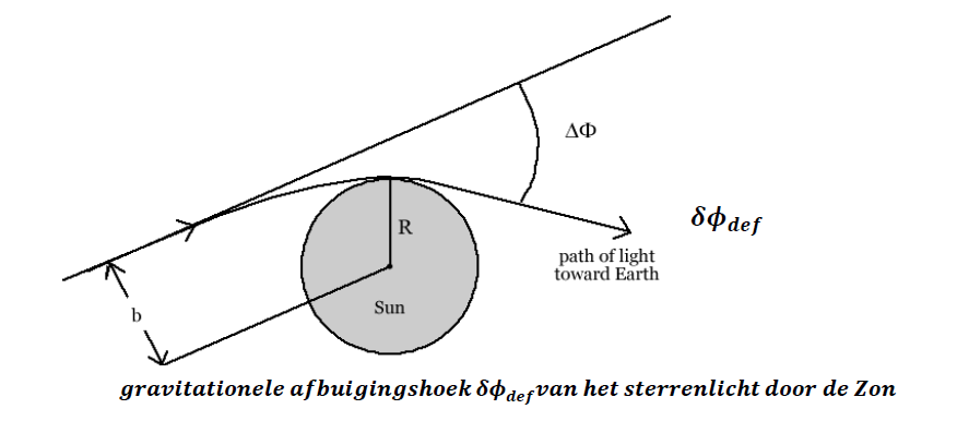
4.3 Experiment 3 - Deflection of Light

4.3.1 Historical and theoretical background

The deflection of light by gravity was the first experimental test of general relativity. In classical Newtonian gravity, light, as a massless phenomenon, travels in straight lines that are not affected by gravity. According to general relativity, however, light follows the curvature of spacetime caused by mass.

As a result, a light ray deviates from a straight line when it passes near a massive object such as the Sun. This effect can be observed when we look at the light from a star that appears visually close to the Sun.

When the light from the star grazes the Sun, it is deflected, so that the star appears at a different position in the sky than where it actually is. Half a year later, when the star is on the opposite side of the sky, its light passes far from the Sun, and its position is observed correctly.

To observe this effect, a solar eclipse is required, because otherwise sunlight overwhelms the starlight. In 1919, this effect was first measured by Arthur Eddington during a total solar eclipse. His observations confirmed Einstein’s prediction and marked a major breakthrough in the acceptance of general relativity.

4.3.2 The derivation of the deflection angle

We consider a light ray (photon) approaching from infinity and passing near the Sun. The motion of the photon in Schwarzschild spacetime is described by the effective energy equation, as derived in chapter 4.2.1.

For a photon, \(\varepsilon = 0\), so:

\begin{align} \frac{1}{2}\left(\frac{dr}{d\lambda}\right)^2 + V(r) = \frac{1}{2}\frac{E^2}{c^2} \label{eq:R182} \end{align}

with:

\begin{align} V(r) = \frac{1}{2}c^2\varepsilon - \varepsilon \frac{GM}{r} + \frac{L^2}{2r^2} - \frac{GM L^2}{c^2 r^3} \label{eq:R183} \end{align}

where \(L\) is the angular momentum and \(E\) the energy of the photon.

For \(\varepsilon = 0\), this yields:

\begin{align} \frac{1}{2}\left(\frac{dr}{d\lambda}\right)^2 + \frac{L^2}{2r^2} - \frac{GM L^2}{c^2 r^3} = \frac{1}{2}\frac{E^2}{c^2} \label{eq:R184} \end{align}

We divide by \(L^2\) and multiply by 2:

\begin{align} \frac{1}{L^2}\left(\frac{dr}{d\lambda}\right)^2 + \frac{1}{r^2} - \frac{2GM}{c^2 r^3} = \frac{E^2}{c^2 L^2} \label{eq:R185} \end{align}

Or equivalently:

\begin{align} \frac{1}{L^2}\left(\frac{dr}{d\lambda}\right)^2 + \frac{1}{r^2} \left(1 - \frac{2GM}{c^2 r}\right) = \frac{E^2}{c^2 L^2} \label{eq:R186} \end{align}

Solving for \(\left(dr/d\lambda\right)^2\) gives:

\begin{align} \left(\frac{dr}{d\lambda}\right)^2 = L^2 \left( \frac{E^2}{c^2 L^2} - \frac{1}{r^2} \left(1 - \frac{2GM}{c^2 r}\right) \right) \label{eq:R187} \end{align}

4.3.3 Impact parameter and angular momentum

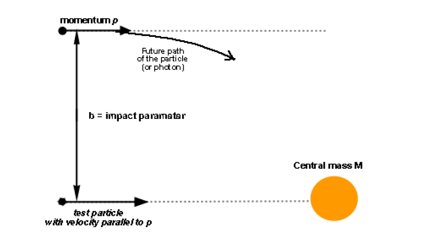
The impact parameter \(b\) is the distance between the line of action of the massive object (the Sun) and the asymptotic direction of the light ray at infinity.

vector_4_3_3
Figure 2. Definition of the impact parameter b. The moving particle approaches the mass M from a large distance with momentum vector p. A test particle with parallel velocity moves radially toward the mass M. The distance b between their initially parallel paths at "infinity" is the impact parameter b.

The angular momentum of the photon is:

\begin{align} L = p\,b \label{eq:R188} \end{align}

For a photon, \(E = pc\), so:

\begin{align} b = \frac{L}{E/c} \label{eq:R189} \end{align}

Additional clarification of the relation (\ref{eq:R188}) and (\ref{eq:R189}):

vector_4_3_3_1

The angular momentum is \(𝐿=𝑝 \, \sin\phi\cdot r=p\cdot r\, \sin\phi \)

The energy in general is \(E^2=p^2 c^2+m^2 c^4 \); and for a photon \(m=0\), so \(E=pc\).
Thus:

\begin{align} \frac{L}{E/c}=\frac{pb}{pc/c}=b \label{eq:R190} \end{align}

It follows:

\begin{align} \frac{1}{b^2} = \frac{E^2}{c^2 L^2} \label{eq:R191} \end{align}

4.3.4 Derivation of the path: the orbit equation for the photon

From the conserved quantity follows:

\begin{align} r^2 \frac{d\phi}{d\lambda} = L \label{eq:R192} \end{align}

Thus:

\begin{align} \frac{d\phi}{d\lambda}=\frac{d\phi}{dr}\frac{dr}{d\lambda}=\frac{L}{r^2} \quad \Rightarrow \quad \frac{d\phi}{dr} = \frac{L}{r^2} \left(\frac{dr}{d\lambda}\right)^{-1} \label{eq:R193} \end{align}

Together with (\ref{eq:R187}) this gives:

\begin{align} \frac{d\phi}{dr}=\frac{L}{r^2}\left(\frac{dr}{d\lambda}\right)^{-1}=\pm \, \frac{L}{r^2} \frac{1}{L}\left[\frac{E^2}{c^2L^2}-\frac{1}{r^2}\left(1-\frac{2GM}{c^2r}\right)\right]^{-1/2} \label{eq:R194} \end{align}

Using (\ref{eq:R191}) this becomes:

\begin{align} \frac{d\phi}{dr} = \pm \frac{1}{r^2} \left( \frac{1}{b^2} - \frac{1}{r^2} \left(1 - \frac{2GM}{c^2 r}\right) \right)^{-1/2} \label{eq:R195} \end{align}

This leads to:

\begin{align} \left(\frac{1}{r^2}\frac{dr}{d\phi}\right)^2 = \frac{1}{b^2} - \frac{1}{r^2} \left(1 - \frac{2GM}{c^2 r}\right) \label{eq:R196} \end{align}

4.3.5 Integration of the path

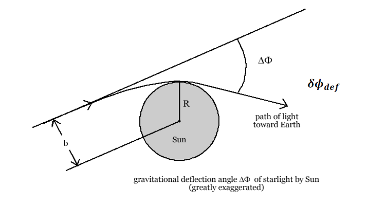
The deflection angle is obtained by calculating the angular change \(\Delta \phi\) along the photon’s trajectory, from infinity to the perihelion \(r = R\), and back. From equation (\ref{eq:R195}) we obtain (see Figure 3):

\begin{align} \Delta \phi = 2 \int_{r_1}^{\infty} \frac{dr}{r^2 \sqrt{ \frac{1}{b^2} - \frac{1}{r^2} \left( 1 - \frac{2GM}{c^2 r} \right) }} \label{eq:R197} \end{align}
vector_4_3_5_1
Fig. 3 - Deflection of light by angle \(\delta \varphi_{def}\)

At the turning point \(r = R\) we have:

\begin{align} \frac{dr}{d\phi} = 0 \label{eq:R198} \end{align}
so from equation (\ref{eq:R196}) follows:

\begin{align} \frac{1}{b^2} = \frac{1}{R^2} \left( 1 - \frac{2GM}{c^2 R} \right) \label{eq:R199} \end{align}

Substitute this into equation (\ref{eq:R196}):

\begin{align} \left( \frac{1}{r^2} \frac{dr}{d\phi} \right)^2 = \frac{1}{R^2} \left( 1 - \frac{2GM}{c^2 R} \right) - \frac{1}{r^2} \left( 1 - \frac{2GM}{c^2 r} \right) \label{eq:R200} \end{align}

4.3.6 Variable substitution

Introduce the substitution:

\begin{align} u = \frac{R}{r} \label{eq:R201} \end{align}

Then:

\begin{align} \frac{du}{d\phi} = \frac{du}{dr} \frac{dr}{d\phi} = - \frac{R}{r^2} \frac{dr}{d\phi} \label{eq:R202} \end{align}
\begin{align} \left( \frac{du}{d\phi} \right)^2 = \frac{R^2}{r^4} \left( \frac{dr}{d\phi} \right)^2 \label{eq:R203} \end{align}

Here \(u\) varies between \(1\) (at \(r = R\)) and \(0\) (at \(r = \infty\)). Equation (\ref{eq:R199}) becomes:

\begin{align} \left( \frac{du}{d\phi} \right)^2 = \left( 1 - \frac{2GM}{c^2 R} \right) - u^2 \left( 1 - \frac{2GM}{c^2 R} u \right) \label{eq:R204} \end{align}

Or:

\begin{align} \left( \frac{du}{d\phi} \right)^2 = 1 - u^2 - \frac{2GM}{c^2 R} \left( 1 - u^3 \right) \label{eq:R205} \end{align}

From this follows:

\begin{align} d\phi = \left[ 1 - u^2 - \frac{2GM}{c^2 R} \left( 1 - u^3 \right) \right]^{-1/2} du \label{eq:R206} \end{align}
\begin{align} =\frac{\left(1-u^2\right)^{-1/2}}{\left[1-\frac{2GM}{c^2R}\left(1-u^3\right) \left(1-u^2\right)^{-1}\right]^{1/2}}\,du \label{eq:R207} \end{align}

This integral is difficult to solve in closed form. To simplify it, we use the substitution:

\begin{align} u = \cos \alpha, \qquad 0 < \alpha < \frac{\pi}{2} \quad thus \quad 0 < u < 1 \label{eq:R208} \end{align}

Then:

\begin{align} d\phi = - \left[ 1 - \frac{2GM}{c^2 R} \frac{1 - \cos^3 \alpha}{\sin^2 \alpha} \right]^{-1/2} d\alpha \label{eq:R209} \end{align}

Noting that:

\begin{align} \frac{1 - \cos^3 \alpha}{\sin^2 \alpha} = \frac{(1 - \cos \alpha)(1 + \cos \alpha + \cos^2 \alpha)} {(1 - \cos \alpha)(1 + \cos \alpha)} = \frac{1 + \cos \alpha + \cos^2 \alpha}{1 + \cos \alpha} \label{eq:R210} \end{align}
\begin{align} =\frac{1 + \cos \alpha \left(1 + \cos \alpha\right)}{1 + \cos \alpha}=\cos \alpha+\frac{1}{1 + \cos \alpha} \label{eq:R211} \end{align}

we finally obtain:

\begin{align} d\phi = - \left[ 1 - \frac{2GM}{c^2 R}\left(\cos\alpha+\frac{1}{1+\cos\alpha}\right) \right]^{-1/2} d\alpha \label{eq:R212} \end{align}

With:

\begin{align} \cos \alpha = \frac{R}{r} \label{eq:R213} \end{align}

Up to this point, no approximation has been applied. This full derivation is suitable for computing the light deflection exactly, although in practice a first-order approximation is often sufficient to determine the deflection angle near the edge of the Sun.

4.3.6.1 Approximations and integration

The parameter

\begin{align} \frac{2GM}{c^2 R} \approx 4.24 \times 10^{-6} \label{eq:R214} \end{align}
is very small at the surface of the Sun.

We apply the Taylor approximation:

\begin{align} \frac{1}{\sqrt{1 - k}} \approx 1 + \frac{1}{2} k \label{eq:R215} \end{align}

Applied to equation (\ref{eq:R213}) this yields:

\begin{align} d\phi = - \left[ 1 - \frac{2GM}{c^2 R}\left(\cos\alpha+\frac{1}{1+\cos\alpha}\right) \right]^{-1/2} d\alpha \label{eq:R216} \end{align}

Or:

\begin{align} d\phi = -\frac{1}{\sqrt{\left[ 1 - \frac{2GM}{c^2 R}\left(\cos\alpha+\frac{1}{1+\cos\alpha}\right) \right]}}d\alpha \label{eq:R217} \end{align}

After approximation:

\begin{align} d\phi \approx - \left[ 1 + \frac{GM}{c^2 R} \left(\cos \alpha+\frac{1}{1 + \cos \alpha}\right) \right] d\alpha \label{eq:R218} \end{align}

We can now compute the total change in azimuth along the full trajectory of the photon, from \(\alpha=0\) to \(\alpha=\frac{\pi}{2}\), and double it:

The total angular change is then:

\begin{align} \Delta \phi = 2 \int_{0}^{\pi/2} \left[ 1 + \frac{GM}{c^2 R} \left(\cos \alpha+\frac{1}{1 + \cos \alpha}\right) \right] d\alpha \label{eq:R219} \end{align}
To evaluate this integral, we consider the second term separately. We consider the integral:
\begin{align} \int \frac{1}{1+\cos\alpha}\, d\alpha \label{eq:R220} \end{align}
We use the trigonometric identity:
\begin{align} 1+\cos\alpha = 1 + \cos\left(\frac{\alpha}{2} + \frac{\alpha}{2}\right) = \cos^2\frac{\alpha}{2} + \sin^2\frac{\alpha}{2} + \cos^2\frac{\alpha}{2} - \sin^2\frac{\alpha}{2} = 2\cos^2\frac{\alpha}{2}. \label{eq:R221} \end{align}
Thus:
\begin{align} \frac{1}{1+\cos\alpha} = \frac{1}{2\cos^2\frac{\alpha}{2}}. \label{eq:R222} \end{align}
Note that:
\begin{align} \frac{1}{2\cos^2\frac{\alpha}{2}} = \frac{1}{2}\left(1+\frac{\sin^2\frac{\alpha}{2}}{\cos^2\frac{\alpha}{2}} \right) = \frac{1}{2}\left( \frac{\cos\frac{\alpha}{2}}{\cos\frac{\alpha}{2}} + \frac{\sin^2\frac{\alpha}{2}}{\cos^2\frac{\alpha}{2}} \right) = \frac{1}{2}\frac{d}{d(\alpha/2)}\tan\frac{\alpha}{2} = \frac{d}{d\alpha}\left(\tan\frac{\alpha}{2}\right). \label{eq:R223} \end{align}
Thus:
\begin{align} \int \frac{1}{1+\cos\alpha}\, d\alpha = \tan\frac{\alpha}{2}. \label{eq:R224} \end{align}

We can now evaluate the full integral (\ref{eq:R219}):

\begin{align} \Delta \phi = 2 \left[ \alpha + \frac{GM}{c^2 R} \left( \sin \alpha + \tan \frac{\alpha}{2} \right) \right]_{0}^{\pi/2} \label{eq:R225} \end{align}
Substituting:
\begin{align} \alpha = \frac{\pi}{2}: &\qquad \sin\frac{\pi}{2} = 1,\qquad \tan\frac{\pi}{4} = 1 \label{eq:R226} \end{align}
\begin{align} \alpha = 0: &\qquad \sin 0 = 0,\qquad \tan 0 = 0 \label{eq:R226a} \end{align}
Thus:
\begin{align} \Delta\phi = 2\left( \frac{\pi}{2} + \frac{GM}{c^{2}R}(1 + 1) \right) = \pi + \frac{4GM}{c^{2}R}. \label{eq:R227} \end{align}
\begin{align} \Delta \phi = \pi + \frac{4GM}{c^2 R} \label{eq:R228} \end{align}

Note: the integral should run from \(r=\infty\) to R, so \(u\) goes from 0 to 1, and thus \(\alpha\) from \(\frac{\pi}{2}\) to 0. By changing the integral to run from 0 to \(\frac{\pi}{2}\), the sign changes and the minus sign disappears.

vector_4_3_6_1

The first term, \(\pi\), is the total angular change of a photon in flat spacetime – a straight trajectory without deflection. The second term is the additional deflection due to spacetime curvature. The actual deflection angle is therefore:

\begin{align} \delta \phi_{\mathrm{def}} = \Delta \phi - \pi \approx \frac{4GM}{c^2 R} \label{eq:R229} \end{align}

Numerical value

With:
\begin{align} \begin{aligned} G &= 6.674 \cdot 10^{-11}\ \mathrm{N\,m^{2}/kg^{2}},\\ M_{s} &= 1.989 \cdot 10^{30}\ \mathrm{kg},\\ c &= 3.00 \cdot 10^{8}\ \mathrm{m/s},\\ R_{s} &= 6.963 \cdot 10^{8}\ \mathrm{m}, \end{aligned} \label{eq:R230} \end{align}
we find:
\begin{align} \delta\phi_{\mathrm{def}} = \frac{4GM_{s}}{c^{2}R_{s}} = \frac{4 \cdot 6.674\cdot 10^{-11} \cdot 1.989\cdot 10^{30}} {(3.00\cdot 10^{8})^{2} \cdot 6.963\cdot 10^{8}} \approx 8.5 \cdot 10^{-6}\ \text{radians}. \label{eq:R231} \end{align}
To convert this into arcseconds, we use:
\begin{align} 1\ \text{rad} = \frac{180 \cdot 60 \cdot 60}{\pi} \approx 206.265''. \label{eq:R232} \end{align}
From this follows:
\begin{align} \delta\phi_{\mathrm{def}} \approx 8.5 \cdot 10^{-6} \times 206.265'' \approx 1.75''. \label{eq:R233} \end{align}

4.3.7 Conclusion

This deflection of 1.75 arcseconds was first observed by Arthur Eddington during the solar eclipse of 1919. The result confirmed, in a spectacular way, Einstein’s prediction and marked a milestone in the experimental verification of general relativity.

This effect is also observed outside our solar system and is known as “gravitational lensing”.

4.3.8 Physical interpretation

  • Light follows the curvature of spacetime.
  • The deflection is a geometric effect, not a force.
  • Observable during solar eclipses.

4.4 Experiment 4 – Precession of the Perihelia (Mercury)

Based on the article by Owen Biesel (Biesel, 2008).
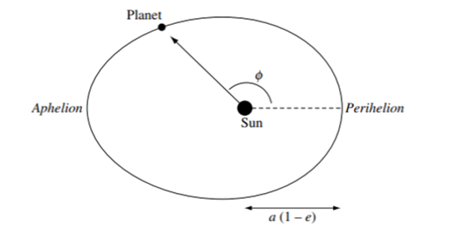
4.4.1 Introduction

  • Physical problem: The orbit of Mercury around the Sun is an ellipse, but the closest point (perihelion) slowly shifts over time. This phenomenon is called perihelion precession.
  • Classical explanation: Newtonian mechanics explains most of this precession (due to the influence of other planets), but a residual of about 43 arcseconds per century remains unexplained.
  • Relativistic explanation: General relativity predicts an additional precession as a result of spacetime curvature around the Sun, exactly matching the observed excess.

4.4.2 Theoretical framework: Schwarzschild metric

In general relativity, we consider a planet such as Mercury as a test particle moving along a geodesic in curved spacetime.

The Schwarzschild metric describes this spacetime around a spherically symmetric mass (such as the Sun):

\begin{align} ds^{2} = c^{2} d\tau^{2} = \sigma^{2} c^{2} dt^{2} - \frac{dr^{2}}{\sigma^{2}} - r^{2} d\theta^{2} - r^{2} \sin^{2}\theta \, d\phi^{2} \label{eq:R234} \end{align}

with:

\begin{align} \sigma = \sqrt{1 - \frac{2GM}{c^{2} r}} = \sqrt{1 - \frac{R_{s}}{r}}, \qquad R_{s} = \frac{2GM}{c^{2}} \label{eq:R235} \end{align}

For a planet moving in the equatorial plane \(\left( \theta = \frac{\pi}{2}\right) \) this simplifies to:

\begin{align} 1 = \left(1 - \frac{R_{s}}{r}\right) \left(\frac{dt}{d\tau}\right)^{2} - \frac{1}{c^{2}} \left(1 - \frac{R_{s}}{r}\right)^{-1} \left(\frac{dr}{d\tau}\right)^{2} - \frac{1}{c^{2}} r^{2} \left(\frac{d\phi}{d\tau}\right)^{2} \label{eq:R236} \end{align}

4.4.3 Derivation via the precession using the Lagrangian approach (see Appendix 12)

Although we have previously derived the expressions for the energy E (equation (\ref{eq:R140})) and the angular momentum L (equation (\ref{eq:R147})), we repeat the derivation here using the Lagrangian. We parametrize the trajectory as:

\begin{align} x^{\mu}(\tau) = \bigl( t(\tau), r(\tau), \theta(\tau), \phi(\tau) \bigr) \label{eq:R237} \end{align}

with \(\tau\) the proper time. In the equatorial plane \(\theta =\frac{\pi}{2}\), the Lagrangian becomes:

\begin{align} \mathcal{L} = \left(1 - \frac{R_{s}}{r}\right) \left(\frac{dt}{d\tau}\right)^{2} - \frac{1}{c^{2}} \left(1 - \frac{R_{s}}{r}\right)^{-1} \left(\frac{dr}{d\tau}\right)^{2} - \frac{1}{c^{2}} r^{2} \left(\frac{d\phi}{d\tau}\right)^{2} \label{eq:R238} \end{align}

The Euler–Lagrange equations for ∅ and t give:

\begin{align} \frac{d\phi}{d\tau} = \dot{\phi}, \qquad \frac{dt}{d\tau} = \dot{t}. \label{eq:R239} \end{align}

The Lagrangian then becomes:

\begin{align} \mathcal{L} = \left(1 - \frac{R_s}{r}\right)\dot{t}^{\,2} - \frac{1}{c^{2}}\left(1 - \frac{R_s}{r}\right)^{-1}\dot{r}^{\,2} - \frac{1}{c^{2}}\, r^{2}\dot{\phi}^{\,2}. \label{eq:R240} \end{align}

4.4.4 Euler–Lagrange operation

Here for \( \phi \):

\begin{align} \frac{d}{d\tau}\left( \frac{\partial \mathcal{L}}{\partial \dot{\phi}} \right) = \frac{\partial \mathcal{L}}{\partial \phi} = 0, \label{eq:R241} \end{align}

and for \( t \):

\begin{align} \frac{d}{d\tau}\left( \frac{\partial \mathcal{L}}{\partial \dot{t}} \right) = \frac{\partial \mathcal{L}}{\partial t} = 0. \label{eq:R242} \end{align}

Then the Euler–Lagrange equations for \( \phi \) and \( t \) are:

\begin{align} 0 = \frac{d}{d\tau}\left(2 \frac{1}{c^{2}} r^{2}\frac{d\phi}{d\tau} \right) \quad\Rightarrow\quad r^{2}\frac{d\phi}{d\tau} = \text{constant} = L, \label{eq:R243} \end{align}
\begin{align} 0 = \frac{d}{d\tau}\left[ 2\left(1 - \frac{R_s}{r}\right)\frac{dt}{d\tau} \right] \quad\Rightarrow\quad \left(1 - \frac{R_s}{r}\right)\frac{dt}{d\tau} = \text{constant} = \frac{E}{c^{2}}. \label{eq:R244} \end{align}

From this it follows that \( L \) (angular momentum per unit mass) and \( E \) (energy per unit mass) are constants of motion.

We rewrite the original normalization condition.

The normalization condition is:

\begin{align} 1 = \left(1 - \frac{R_s}{r}\right)\left(\frac{dt}{d\tau}\right)^{2} - \frac{1}{c^{2}}\left(1 - \frac{R_s}{r}\right)^{-1}\left(\frac{dr}{d\tau}\right)^{2} - \frac{1}{c^{2}} r^{2}\left(\frac{d\phi}{d\tau}\right)^{2}. \label{eq:R245} \end{align}

We substitute the constants \(E\) and \(L\):

\begin{align} 1 = \frac{\frac{E^{2}}{c^{4}}}{1-\frac{R_s}{r}} - \frac{1}{c^{2}}\frac{\left(\frac{dr}{d\tau}\right)^{2}}{1 - \frac{R_s}{r}} - \frac{L^{2}}{c^{2} r^{2}}. \label{eq:R246} \end{align}
\begin{align} 1 - \frac{R_s}{r} = \frac{E^{2}}{c^{4}} - \frac{1}{c^{2}}\left(\frac{dr}{d\tau}\right)^{2} - \frac{L^{2}}{c^{2}r^{2}} + \frac{R_s L^{2}}{c^{2} r^{3}}. \label{eq:R247} \end{align}

Thus:

\begin{align} \left(\frac{dr}{d\tau}\right)^{2} = c^{2}\left(\frac{E^{2}}{c^{4}} - 1\right) + c^{2}\frac{R_s}{r} - \frac{L^{2}}{r^{2}} + \frac{R_s L^{2}}{r^{3}}. \label{eq:R248} \end{align}

By:

\begin{align} \frac{dr}{d\tau} = \frac{dr}{d\tau} = \frac{dr}{d\phi}\frac{d\phi}{d\tau} = \frac{dr}{d\phi}\frac{L}{r^{2}} \quad\Rightarrow\quad \left(\frac{dr}{d\phi}\right)^{2} = \frac{r^{4}}{L^{2}}\,\left(\frac{dr}{d\tau}\right)^{2}, \label{eq:R249} \end{align}

we obtain:

\begin{align} \left(\frac{dr}{d\phi}\right)^{2} = \frac{r^{4}}{L^{2}} \left[ c^{2}\left(\frac{E^{2}}{c^{4}} - 1\right) + c^{2}\frac{R_s}{r} - \frac{L^{2}}{r^{2}} + \frac{R_s L^{2}}{r^{3}} \right]. \label{eq:R250} \end{align}

This can be written as:

\begin{align} \left(\frac{dr}{d\phi}\right)^{2} = \text{Newtonian terms} \;+\; \text{relativistic correction}. \label{eq:R251} \end{align}

The extra term \( \frac{R_s L^{2}}{r^{3}} \) in the effective potential causes the precession of the perihelion.

After simplification:

\begin{align} \left(\frac{dr}{d\phi}\right)^{2} = \frac{c^{2}}{L^{2}}\left(\frac{E^{2}}{c^{4}} - 1\right) r^{4} + \frac{c^{2}R_s}{L^2} r^{3} - r^{2} + R_s r. \label{eq:R252} \end{align}

From this we derive:

\begin{align} d\phi = \frac{dr}{ \sqrt{ \frac{c^{2}}{L^{2}}\left(\frac{E^{2}}{c^{4}} - 1\right) r^{4} + \frac{c^{2}R_s}{L^2} r^{3} - r^{2} + R_s r }}. \label{eq:R253} \end{align}

4.4.5 Precession of the Orbit

For a closed orbit, the radial motion must be bounded, i.e. \(dr/d\phi=0\) at two points: the perihelion P and the aphelion A. However, for a non-closed orbit (precession), the angular shift between perihelion \(P\) and aphelion \(A\) is:

\begin{align} \phi_{A} - \phi_{P} = \int_{P}^{A} \frac{dr}{ \sqrt{ \frac{c^{2}}{L^{2}} \left(\frac{E^{2}}{c^{4}} - 1\right) r^{4} + \frac{c^{2} R_{s}}{L^2} r^{3} - r^{2} + R_{s} r } } \label{eq:R254} \end{align}

To express \(E\) and \(L\) in terms of \(A\), \(P\), and \(R_s\), we impose that \(\frac{dr}{d\phi}=0\) for \(r=A\) and \(r=P\). This leads to the following equations:

\begin{align} c^{2}\left(\frac{E^{2}}{c^{4}} - 1\right)A^{4} + L^{2}(- A^{2}+ R_{s}A) = -c^{2}R_{s}A^{3} \label{eq:R255} \end{align}
\begin{align} c^{2}\left(\frac{E^{2}}{c^{4}} - 1\right)P^{4} + L^{2}(- P^{2}+ R_{s}P) = -c^{2}R_{s}P^{3} \label{eq:R256} \end{align}

By taking suitable combinations and subtractions of these equations, we can fully express \(\frac{E^{2}}{c^{4}} - 1\) and \(L^{2}\) in terms of \(A\), \(P\), and \(R_s\). (See the original derivation for details.)

Multiply (\ref{eq:R255}) by \((-P^{2}+R_{s}P)\):

\begin{align} c^{2}\left(\frac{E^{2}}{c^{4}} - 1\right)A^{4}(-P^{2}+R_{s}P) + L^{2}(-A^{2}+R_{s}A)(-P^{2}+R_{s}P) = -c^{2}R_{s}A^{3}(-P^{2}+R_{s}P) \label{eq:R257} \end{align}

Multiply (\ref{eq:R256}) by \((-A^{2}+R_{s}A)\):

\begin{align} c^{2}\left(\frac{E^{2}}{c^{4}} - 1\right)P^{4}(-A^{2}+R_{s}A) + L^{2}(-P^{2}+R_{s}P)(-A^{2}+R_{s}A) = -c^{2}R_{s}P^{3}(-A^{2}+R_{s}A) \label{eq:R258} \end{align}

Subtract these two equations:

\begin{align} c^{2}\left(\frac{E^{2}}{c^{4}} - 1\right) \left[ A^{4}(-P^{2}+R_{s}P) - P^{4}(-A^{2}+R_{s}A) \right] = -c^{2}R_{s}A^{3}(-P^{2}+R_{s}P) + c^{2}R_{s}P^{3}(-A^{2}+R_{s}A) \label{eq:R259} \end{align}

From this follows:

\begin{align} c^{2}\left(\frac{E^{2}}{c^{4}} - 1\right) = \frac{ -c^{2}R_{s}A^{3}(-P^{2}+R_{s}P) + c^{2}R_{s}P^{3}(-A^{2}+R_{s}A) }{ A^{4}(-P^{2}+R_{s}P) - P^{4}(-A^{2}+R_{s}A) } \label{eq:R260} \end{align}

Thus:

\begin{align} \frac{E^{2}}{c^{4}} - 1 = \frac{ -R_{s}A^{3}(-P^{2}+R_{s}P) + R_{s}P^{3}(-A^{2}+R_{s}A) }{ [A^{4}(-P^{2}+R_{s}P) - P^{4}(-A^{2}+R_{s}A)] } \label{eq:R261} \end{align}
\begin{align} \frac{E^{2}}{c^{4}} - 1 = \frac{ -R_{s}[A^{3}(-P^{2}+R_{s}P) - P^{3}(-A^{2}+R_{s}A) }{ [A^{4}(-P^{2}+R_{s}P) - P^{4}(-A^{2}+R_{s}A)] } \label{eq:R262} \end{align}
\begin{align} \frac{E^{2}}{c^{4}} - 1 = \frac{ -R_{s}[A^{3}P(-P+R_{s}) - P^{3}A(-A+R_{s}) }{ [A^{4}P(-P+R_{s}) - P^{4}A(-A+R_{s})] } \label{eq:R263} \end{align}
\begin{align} \frac{E^{2}}{c^{4}} - 1 = \frac{ -R_{s}AP[A^{2}(-P+R_{s}) - P^{2}(-A+R_{s}) }{ AP[A^{3}(-P+R_{s}) - P^{3}(-A+R_{s})] } \label{eq:R264} \end{align}
\begin{align} \frac{E^{2}}{c^{4}} - 1 = \frac{ -R_{s}[A^{2}(-P+R_{s}) - P^{2}(-A+R_{s}) }{ [A^{3}(-P+R_{s}) - P^{3}(-A+R_{s})] } \label{eq:R265} \end{align}
\begin{align} \frac{E^{2}}{c^{4}} - 1 = \frac{ -R_{s}[-PA^{2}+R_{s}A^{2}+AP^2-R_sP^2] }{ [-PA^{3}+R_sA^3+AP^3-R_sP^3] } \label{eq:R266} \end{align}
\begin{align} \frac{E^{2}}{c^{4}} - 1 = \frac{ -R_{s}[-AP(A-P)+R_s(A^2-P^2] }{ [-AP(A^2-P^2)+R_s(A^3-P^3] } \label{eq:R267} \end{align}
\begin{align} \frac{E^{2}}{c^{4}} - 1 = \frac{ -R_{s}(A-P)[-AP+R_s(A+P] }{ (A-P)[-AP(A+P)+R_s\frac{A^3-P^3}{A-P}] } \label{eq:R268} \end{align}

Intermezzo to evaluate \(\frac{A^3-P^3}{A-P}\):

\begin{align} (A^2-P^2)(A+P)=A^3-AP^2+A^2P-P^3 \label{eq:R269} \end{align}
\begin{align} A^3-P^3=(A^2-P^2)(A+P)-AP(A-P) \label{eq:R270} \end{align}
\begin{align} A^3-P^3=(A-P)(A+P)(A+P)-AP(A-P) \label{eq:R271} \end{align}
\begin{align} \Rightarrow\quad \frac{A^3-P^3}{A-P}=(A+P)^2-AP \label{eq:R272} \end{align}

Now we substitute the result:

\begin{align} \frac{E^{2}}{c^{4}} - 1 = \frac{ -R_{s}(A-P)[-AP+R_s(A+P] }{ (A-P)[-AP(A+P)+R_s(A+P)^2-R_sAP] } \label{eq:R273} \end{align}
\begin{align} \frac{E^{2}}{c^{4}} - 1 = \frac{ -R_{s}[-AP+R_s(A+P] }{ [-AP(A+P+R_s)+R_s(A+P)^2] } \label{eq:R274} \end{align}
\begin{align} \frac{E^{2}}{c^{4}} - 1 = \frac{ R_{s}[-AP+R_s(A+P] }{ [AP(A+P+R_s)-R_s(A+P)^2] } \label{eq:R275} \end{align}

We can now find \(L^2/c^2\) by applying the same method to equations (\ref{eq:R255}) and (\ref{eq:R256}):

\begin{align} c^{2}\left(\frac{E^{2}}{c^{4}} - 1\right)A^{4} + L^{2}(- A^{2}+ R_{s}A) = -c^{2}R_{s}A^{3} \label{eq:R276} \end{align}
\begin{align} c^{2}\left(\frac{E^{2}}{c^{4}} - 1\right)P^{4} + L^{2}(- P^{2}+ R_{s}P) = -c^{2}R_{s}P^{3} \label{eq:R277} \end{align}

Multiply (\ref{eq:R255}) by \(P^4\).

\begin{align} c^{2}\left(\frac{E^{2}}{c^{4}} - 1\right)A^{4}P^4 + L^{2}(- A^{2}+ R_{s}A)P^4 = -c^{2}R_{s}A^{3}P^4 \label{eq:R278} \end{align}

Multiply (\ref{eq:R256}) by \(A^4\):

\begin{align} c^{2}\left(\frac{E^{2}}{c^{4}} - 1\right)A^4P^{4} + L^{2}(- P^{2}+ R_{s}P)A^4 = -c^{2}R_{s}A^4P^{3} \label{eq:R279} \end{align}

Now subtract:

\begin{align} L^{2}[(-A^2+R_sA)P^4-(-P^2+R_sP)A^4]=-c^2R_sA^3P^4+c^2R_sA^4P^3 \label{eq:R280} \end{align}
\begin{align} L^2=\frac{c^2R_sA^3P^3(-P+A)}{(-A^2+R_sA)P^4-(-P^2+R_sP)A^4} \label{eq:R281} \end{align}
\begin{align} L^2=\frac{c^2R_sA^3P^3(-P+A)}{(-A+R_s)AP^4-(-P+R_s)PA^4} \label{eq:R282} \end{align}
\begin{align} L^2=\frac{c^2R_sA^3P^3(-P+A)}{AP[(-A+R_s)P^3-(-P+R_s)A^3} \label{eq:R283} \end{align}
\begin{align} L^2=\frac{c^2R_sA^2P^2(-P+A)}{[(-A+R_s)P^3-(-P+R_s)A^3} \label{eq:R284} \end{align}
\begin{align} L^2=\frac{c^2R_sA^2P^2(-P+A)}{A^3P-AP^3-(A^3-P^3)R_s} \label{eq:R285} \end{align}
\begin{align} L^2=\frac{c^2R_sA^2P^2(-P+A)}{AP(A^2-P^2)-(A^3-P^3)R_s} \label{eq:R286} \end{align}
\begin{align} L^2=\frac{c^2R_sA^2P^2}{AP(A+P)-R_s(A+P)^2+APR_s} \label{eq:R287} \end{align}
\begin{align} L^2=\frac{c^2R_sA^2P^2}{AP(A+P+R_s)-R_s(A+P)^2} \label{eq:R288} \end{align}
\begin{align} \frac{L^2}{c^2}=\frac{R_sA^2P^2}{AP(A+P+R_s)-R_s(A+P)^2} \label{eq:R289} \end{align}

Finally, we obtain equation (\ref{eq:R275}) above and the expression for \(L^2/c^2\):

\begin{align} \frac{E^2}{c^4}-1=\frac{-APR_s+(A+P)R_s^2}{AP(A+P+R_s)-R_s(A+P)^2} \label{eq:R290} \end{align}
\begin{align} \frac{L^2}{c^2}=\frac{A^2P^2R_s}{AP(A+P+R_s)-R_s(A+P)^2} \label{eq:R291} \end{align}

Next, we can introduce the variable:

\begin{align} D=\frac{AP}{A+P} \label{eq:R292} \end{align}

to further simplify the expressions. This has the dimension of length. Then the expressions above for \(E^2-1\) and \(L^2\) become:

We previously found:

\begin{align} \frac{E^{2}}{c^{4}} - 1 =\frac{ -\frac{R_{s}}{AP} + \frac{R_{s}^{2}}{D\,AP})} { \frac{1}{D} + \frac{R_{s}}{AP} - \frac{R_{s}}{D^{2}} } \label{eq:R293} \end{align}
\begin{align} \frac{L^{2}}{c^{2}} = \frac{R_{s}}{ \frac{1}{D} + \frac{R_{s}}{AP} - \frac{R_{s}}{D^{2}}} \label{eq:R294} \end{align}

Thus:

\begin{align} \frac{\frac{L^{2}}{c^{2}}}{ \frac{E^{2}}{c^{4}} - 1 } = \frac{R_{s}}{ -\frac{R_{s}}{AP} + \frac{R_{s}^{2}}{D\,AP} } = \frac{AP}{- 1 + R_{s}/D} \label{eq:R295} \end{align}
\begin{align}\frac{ \frac{L^{2}}{c^{2}AP}}{{1 - \frac{E^{2}}{c^{4}}}} = \frac{1}{1 - R_{s}/D} \label{eq:R296} \end{align}

We want an expression for \(\varepsilon\), the third non-zero root of:

\begin{align} \frac{E^{2}/c^{4} - 1}{L^{2}/c^{2}} r^{4} + \frac{R_{s}}{L^2/c^2} r^{3} - r^{2} + R_{s} r = 0 \label{eq:R297} \end{align}
\begin{align} \frac{E^2/c^4-1}{L^2/c^2}\left[r^4+\frac{R_s}{E^2/c^4-1}r^3- \frac{L^2/c^2}{E^2/c^4-1}r^2+\frac{L^2/c^2}{E^2/c^4-1}R_sr \right]=0 \label{eq:R298} \end{align}

This therefore gives the three non-zero roots: A, P and \(\varepsilon\).

The full expression becomes:

\begin{align} \frac{E^2/c^4-1}{L^2/c^2} (r-A)(r-P)(r-\varepsilon) r \label{eq:R299} \end{align}

Let us expand the four factors:

\begin{align} \frac{E^2/c^4-1}{L^2/c^2}\left[ r^{4} - (A+P+\varepsilon)\, r^{3} + \{AP + \varepsilon(A + P)\}\, r^{2} - \varepsilon AP\, r \right] \label{eq:R300} \end{align}

We know that the sum of the three non-zero roots equals \(\dfrac{R_{s}}{E^{2}/c^{4} - 1}\) (the coefficient of \(r^{3}\) in the standard form of the polynomial); therefore we obtain:

\begin{align} -(A+P+\varepsilon) = \frac{R_{s}}{E^{2}/c^{4} - 1} \label{eq:R301} \end{align}

This allows us to further analyze the relation between the roots A, P and \(\varepsilon\) in terms of \(R_{s}\), the Schwarzschild radius, and the energy and angular momentum terms.

From the above we know that:

\begin{align} \frac{E^2}{c^4}-1=\frac{R_s[-AP+(A+P)R_s]}{AP(A+P+R_s)-R_s(A+P)^2} \label{eq:R302} \end{align}

Thus we substitute this into the equation above:

\begin{align} A + P + \varepsilon = \frac{R_{s}}{E^{2}/c^{4} - 1} \label{eq:R303} \end{align}
\begin{align} A + P + \varepsilon = R_s\frac{-AP(A+P+R_s)+R_s(A+P)^2}{R_s[-AP+(A+P)R_s]}=\frac{-AP(A+P+R_s)+R_s(A+P)^2}{-AP+(A+P)R_s} \label{eq:R304} \end{align}
\begin{align} \varepsilon=\frac{-AP(A+P+R_s)+R_s(A+P)^2}{-AP+(A+P)R_s}-(A+P) \label{eq:R305} \end{align}
\begin{align} =\frac{-AP(A+P+R_s)+R_s(A+P)^2+AP(A+P)-(A+P)^2R_s}{-AP+(A+P)R_s} \label{eq:R306} \end{align}
\begin{align} \varepsilon=\frac{-AP(A+P+R_s)+AP(A+P)}{-AP+(A+P)R_s}=\frac{-APR_s}{-AP+(A+P)R_s}= \frac{R_s}{1-\frac{(A+P)R_s}{AP}}=\frac{R_s}{1-\frac{R_s}{D}} \label{eq:R307} \end{align}

This gives:

\begin{align} \varepsilon = R_{s}\left(1 - \frac{R_{s}}{D}\right) \label{eq:R308} \end{align}

We can now approximate (\ref{eq:R254}) by writing

\begin{align} \frac{E^2/c^4-1}{L^2/c^2}r^4 + \frac{R_s}{L^2/c^2}r^3-r^2+R_s r =\frac{E^2/c^4-1}{L^2/c^2} (r-A)(r-P)(r-\varepsilon) r \label{eq:R309} \end{align}
\begin{align} =\frac{1-E^2/c^4}{L^2/c^2} (A-r)(r-P)(r-\varepsilon) r \label{eq:R310} \end{align}

Using equation (\ref{eq:R254}) we obtain:

\begin{align} \phi_{A} - \phi_{P} = \sqrt{\frac{L^{2}/c^{2}}{1 - E^{2}/c^{4}}} \int_{P}^{A} \frac{1}{\sqrt{r(A-r)(r-P)(r-\varepsilon)}}\,dr \label{eq:R311} \end{align}
\begin{align} = \sqrt{\frac{L^{2}/c^{2}}{1 - E^{2}/c^{4}}} \int_{P}^{A} \frac{1}{\sqrt{r^2(A-r)(r-P)(1-\frac{\varepsilon}{r})}}\,dr \label{eq:R312} \end{align}
\begin{align} = \sqrt{\frac{L^{2}/c^{2}}{1 - E^{2}/c^{4}}} \int_{P}^{A} \frac{1}{r\sqrt{(A-r)(r-P)}}(1-\frac{\varepsilon}{r})^{-1/2}\,dr \label{eq:R313} \end{align}

Now we use the Taylor series expansion

\begin{align} (1-\frac{\varepsilon}{ r})^{-1/2} \approx 1 + \frac{\varepsilon}{2 r}, \label{eq:R314} \end{align}

with an error \(\varepsilon\) bounded by:

\begin{align} |\varepsilon| \leq \frac{3}{8}(1-\frac{\varepsilon}{ r})^{-5/2}(\frac{\varepsilon}{ r})^{2} \leq \frac{3}{8}(1-\frac{\varepsilon}{ A})^{-5/2}(\frac{\varepsilon}{ P})^{2} \label{eq:R315} \end{align}

which yields:

\begin{align} \phi_{A} - \phi_{P} = \sqrt{\frac{L^{2}/c^{2}}{1 - E^{2}/c^{4}}} \int_{P}^{A}\left[\frac{1}{r\sqrt{(A-r)(r-P)}} +\frac{\varepsilon/2}{r^2\sqrt{(A-r)(r-P)}} \right]dr \label{eq:R316} \end{align}

Remark:
In his article “The Precession of Mercury’s Perihelion” by Owen Biesel (January 25, 2008), on page 8, the left-hand side of the integral (\ref{eq:R316}) contains \(1+\varepsilon\) in the numerator, but we believe it should be only \(1\), and we have adjusted the formula accordingly.

The first integral of (\ref{eq:R316}) (derivation see 4.4.6.1 and 4.4.6.3) in closed form:

\begin{align} \int_{P}^{A} \frac{1}{r\sqrt{(A-r)(r-P)}}\,dr \label{eq:R317} \end{align}
\begin{align} =\frac{1}{\sqrt{AP}}\arctan{\left[ \frac{(A-r)(r-P)+r^2-AP}{2\sqrt{(A-r)(r-P)AP}} \right]_{P}^{A}} \label{eq:R318} \end{align}
\begin{align} \to \frac{1}{\sqrt{AP}} \left[ \arctan(+\infty) - \arctan(-\infty) \right] = \frac{1}{\sqrt{AP}} \left( \frac{\pi}{2} + \frac{\pi}{2} \right) = \frac{\pi}{\sqrt{AP}} \label{eq:R319} \end{align}

The second integral of (\ref{eq:R316}) (derivation see 4.4.6.2) is more difficult, but can be evaluated in closed form:

\begin{align} \int_P^A \frac{\varepsilon/2}{r^2\sqrt{(A-r)(r-P)}}\,dr = \frac{\pi \varepsilon/2}{2\sqrt{AP}}\frac{A+P}{AP} = \frac{1}{\sqrt{AP}}\frac{\pi \varepsilon}{4D} \label{eq:R320} \end{align}

If we now recognize that:

\begin{align} \frac{L^2/c^2}{AP(1 - E^{2}/c^{4})} = \frac{1}{1 - R_{s}/D} \label{eq:R321} \end{align}

and:

\begin{align} \varepsilon = \frac{R_{s}}{1 - R_{s}/D} \label{eq:R322} \end{align}

(see (\ref{eq:R296}) and (\ref{eq:R308}) above), then we find that:

\begin{align} \phi_{A} - \phi_{P} = \frac{1}{\sqrt{AP}}\pi \sqrt{\frac{L^{2}/c^{2}}{1 - E^{2}/c^{4}}} + \frac{1}{\sqrt{AP}}\frac{\pi \varepsilon}{4D}\sqrt{\frac{L^{2}/c^{2}}{1 - E^{2}/c^{4}}} \label{eq:R323} \end{align}
\begin{align} \phi_{A} - \phi_{P} = \pi \sqrt{\frac{L^{2}/c^{2}}{AP(1 - E^{2}/c^{4})}} + \frac{\pi\varepsilon}{4D}\sqrt{\frac{L^{2}/c^{2}}{AP(1 - E^{2}/c^{4})}} \label{eq:R324} \end{align}
\begin{align} \phi_{A} - \phi_{P} = \pi \sqrt{\frac{1}{1 - R_{s}/D}} + \frac{\pi\varepsilon}{4D}\sqrt{\frac{1}{1 - R_{s}/D}} \label{eq:R325} \end{align}
\begin{align} = \frac{\pi}{\sqrt{1 - R_{s}/D}} \left( 1 + \frac{\varepsilon}{4D} \right) \label{eq:R326} \end{align}
\begin{align} = \frac{\pi}{\sqrt{1 - R_{s}/D}} \left( 1 + \frac{1}{4D}\frac{R_{s}}{1 - R_{s}/D} \right) \label{eq:R327} \end{align}
\begin{align} = \frac{\pi}{\sqrt{1 - R_{s}/D}} \left( 1 + \frac{1}{4}\frac{R_{s}/D}{1 - R_{s}/D} \right) \label{eq:R328} \end{align}

Using the observed values \(A\text{(aphelion)} = 69.8 \cdot 10^{6}\,\text{km}\), and \(P\text{(perihelion)} = 46.0 \cdot 10^{6}\,\text{km}\), we obtain:

\begin{align} D = 27.7 \cdot 10^{6}\,\text{km}, \qquad R_{s} = \frac{2GM}{c^{2}} = 2.95\,\text{km} \label{eq:R329} \end{align}

We can then approximate the expression as follows:

\begin{align} \frac{\pi}{\sqrt{1 - R_{s}/D}} \left( 1 + \frac{1}{4}\frac{R_{s}/D}{1 - R_{s}/D} \right) \approx \pi + 2.512 \cdot 10^{-7} \label{eq:R330} \end{align}

This yields a reliable estimate of \(\phi_{A} - \phi_{P}\) (half a revolution, in radians).

This gives:

\begin{align} \Delta \phi = 2.512 \cdot 10^{-7} \text{ radians (half revolution)} \label{eq:R331} \end{align}

And:

\begin{align} \Delta \phi = 5.024 \cdot 10^{-7} \text{ radians (full revolution)} \label{eq:R332} \end{align}

The orbital period of Mercury is 87.969 days, so Mercury completes 415.2 revolutions per century. Since there are \( 360 \cdot 60 \cdot 60/2\pi \) arcseconds per radian, we find that the perihelion of Mercury shifts by:

\begin{align} \Delta \phi = 5.024 \cdot 10^{-7} \cdot \frac{360 \cdot 60 \cdot 60}{2\pi} \cdot \text{415.2} = \text{43.027 arcseconds per century} \label{eq:R333} \end{align}
\begin{align} \Delta \phi = \mathbf{43.027\ arcseconds\ per\ century.} \label{eq:R334} \end{align}

Remark:

According to Asaf Pe'er, for a small deflection angle, the result (see equation (\ref{eq:R547}) chapter 4.7):

\begin{align} \delta \phi_{\text{prec}} = \frac{6\pi G M_{\text{sun}}}{c^{2} a (1 - \varepsilon^{2})} \label{eq:R335} \end{align}

For Mercury:

  • \(a\) is the semi-major axis: \(5.79 \times 10^{10}\,\text{m}\)
  • \(\varepsilon\) is the eccentricity: \(0.206\)
  • \(M\) is the mass of the Sun: \(1.989 \times 10^{30}\,\text{kg}\)
  • \(G\) is the gravitational constant: \(6.674 \times 10^{-11}\,\text{Nm}^{2}\text{kg}^{-2}\)
  • \(c\) is the speed of light: \(3 \times 10^{8}\,\text{m/s}\)
\begin{align} \Delta \phi = \frac{6\pi G M}{a(1 - e^{2})c^{2}} = 5.02 \times 10^{-7}\ \text{rad per revolution} \label{eq:R336} \end{align}

To compute the precession per century:

\begin{align} \Delta \phi = 5.02 \times 10^{-7} \times 100 \times \text{365.2588} \times \frac{360 \times 60 \times 60}{2\pi} \label{eq:R337} \end{align}
\begin{align} \Delta \phi = \mathbf{43''} \text{ arcseconds per century.} \label{eq:R338} \end{align}

Which leads to the same result.

This gives us the exact relation for the precession angle of Mercury’s orbit, as described in the result of 43.027 arcseconds per century.

To express \(E\) and \(L\) in terms of \(A\), \(P\), and \(R_s\), we impose \(\frac{dr}{d\phi}=0\) for \(r=A\) and \(r=P\). This leads to the following equations:

4.4.6 Conclusion

The deviation of Mercury’s orbit due to general relativity is determined by the additional curvature terms in equation (\ref{eq:R254}). The actual precession per orbit can be computed from the deviation of the integral \(\Delta \phi\) relative to \(2\pi\). This theoretical prediction agrees with the observed deviation of approximately 43 arcseconds per century, an effect that cannot be explained by Newtonian mechanics.

4.4.6.1 Verification of the first integral

Verification of the integrand:

\begin{align} \frac{d}{dr} \left[ \frac{1}{\sqrt{AP}} \arctan \left( \frac{(A - r)(r - P)+r^2-AP} {2\sqrt{(A-r)(r-P)AP}} \right) \right] \stackrel{?}{=} \frac{1}{r\sqrt{(A - r)(r - P)}} \label{eq:R340} \end{align}

We know that:

\begin{align} \frac{d}{dx} \arctan x = \frac{1}{1 + x^{2}} \label{eq:R341} \end{align}

Therefore:

\begin{align} \frac{1}{\sqrt{AP}}\frac{d}{dr} \left[ \arctan\left(\frac{(A-r)(r-P)+r^2-AP}{2\sqrt{(A-r)(r-P)AP}}\right) \right] \label{eq:R342} \end{align}
\begin{align} = \frac{1}{\sqrt{AP}} \frac{1}{1+\left(\frac{(A-r)(r-P)+r^2-AP}{2\sqrt{(A-r)(r-P)AP}}\right)^2} \frac{d}{dr} \left[\frac{(A-r)(r-P)+r^2-AP}{2\sqrt{(A-r)(r-P)AP}}\right] \label{eq:R343} \end{align}
\begin{align} = \frac{1}{\sqrt{AP}} \frac{4(A-r)(r-P)AP}{4(A-r)(r-P)AP+[(A-r)(r-P)+r^2-AP]^2} \frac{d}{dr} \left[\frac{(A-r)(r-P)+r^2-AP}{2\sqrt{(A-r)(r-P)AP}}\right] \label{eq:R344} \end{align}
\begin{align} \begin{aligned} &=\frac{1}{\sqrt{AP}} \frac{4(A-r)(r-P)AP}{4(A-r)(r-P)AP+[(A-r)(r-P)+r^2-AP]^2}\cdot \\ \notag &\quad \left[\frac{-(r-P)+(A-r)+2r}{2\sqrt{(A-r)(r-P)AP}} -\frac{AP{(A-r)(r-P)+r^2-AP}{-(r-P)+(A-r)}}{4{(A-r)(r-P)AP}^{3/2}}\right] \end{aligned} \label{eq:R345} \end{align}
\begin{align} \begin{aligned} &=\frac{1}{\sqrt{AP}} \frac{4(A-r)(r-P)AP}{4(A-r)(r-P)AP+[(A-r)(r-P)+r^2-AP]^2}\cdot \\ \notag &\quad \left[\frac{A+P}{2\sqrt{(A-r)(r-P)AP}} -\frac{AP{(A-r)(r-P)+r^2-AP}{-(r-P)+(A-r)}}{4{(A-r)(r-P)AP}^{3/2}}\right] \end{aligned} \label{eq:R346} \end{align}
\begin{align} \begin{aligned} &=\frac{1}{\sqrt{AP}} \frac{4(A-r)(r-P)AP}{4(A-r)(r-P)AP+[(A-r)(r-P)+r^2-AP]^2}\cdot \\ \notag &\quad \left[\frac{A+P}{2\sqrt{(A-r)(r-P)AP}} -\frac{AP{(Ar-2AP+rP)(P+A-2r)}}{4[{(A-r)(r-P)AP}]^{3/2}}\right] \end{aligned} \label{eq:R347} \end{align}
\begin{align} \begin{aligned} &=\frac{1}{\sqrt{AP}} \frac{4(A-r)(r-P)AP}{4(A-r)(r-P)AP+[(A-r)(r-P)+r^2-AP]^2}\frac{1}{\sqrt{(A-r)(r-P)AP}}\cdot \\ \notag &\quad \left[\frac{2(A+P)}{4} -\frac{AP{(Ar-2AP+rP)(P+A-2r)}}{4(A-r)(r-P)AP}\right] \end{aligned} \label{eq:R348} \end{align}
\begin{align} \begin{aligned} &=\frac{1}{\sqrt{AP}} \frac{4(A-r)(r-P)AP}{4(A-r)(r-P)AP+[(A-r)(r-P)+r^2-AP]^2}\frac{1}{\sqrt{(A-r)(r-P)AP}}\cdot \\ \notag &\quad \left[\frac{2(A+P)(A-r)(r-P)AP-AP(Ar-2AP+rP)(P+A-2r)}{4(A-r)(r-P)AP} \right] \end{aligned} \label{eq:R349} \end{align}
\begin{align} =\frac{1}{\sqrt{AP}} \frac{2(A+P)(A-r)(r-P)AP-AP(Ar-2AP+rP)(P+A-2r)}{4(A-r)(r-P)AP+[(A-r)(r-P)+r^2-AP]^2} \frac{1}{\sqrt{(A-r)(r-P)AP}} \label{eq:R350} \end{align}
\begin{align} =\frac{1}{AP\sqrt{(A-r)(r-P)}} \frac{2(A+P)(A-r)(r-P)AP-AP(Ar-2AP+rP)(P+A-2r)}{4(A-r)(r-P)AP+[(A-r)(r-P)+r^2-AP]^2} \label{eq:R351} \end{align}
\begin{align} =\frac{1}{\sqrt{(A-r)(r-P)}} \frac{2(A+P)(A-r)(r-P)-(Ar-2AP+rP)(P+A-2r)}{4(A-r)(r-P)AP+[(A-r)(r-P)+r^2-AP]^2} \label{eq:R352} \end{align}
\begin{align} =\frac{1}{\sqrt{(A-r)(r-P)}} \frac{(2A^2-2Ar+2AP-2Pr)(r-P)-(APr-2AP^2+rP^2+A^2r-2A^2P+APr-2Ar^2+4APr-2Pr^2)} {4A^2Pr-4APr^2-4A^2P^2+4AP^2r+[Ar-r^2-AP+Pr+r^2-AP]^2} \label{eq:R353} \end{align}
\begin{align} =\frac{1}{\sqrt{(A-r)(r-P)}} \frac{(2A^2-2Ar+2AP-2Pr)(r-P)-(6APr-2AP^2+P^2r+A^2r-2A^2P-2Ar^2-2Pr^2)} {4A^2Pr-4APr^2-4A^2P^2+4AP^2r+[Ar-2AP+Pr]^2} \label{eq:R354} \end{align}
\begin{align} =\frac{1}{\sqrt{(A-r)(r-P)}} \frac{2A^2-2Ar+4APr-2Pr^2-2A^2P-2AP^2+2P^2r-6APr+2AP^2-P^2r-A^2r+2A^2P+2Ar^2+2Pr^2} {4A^2Pr-4APr^2-4A^2P^2+4AP^2r+[Ar-2AP+Pr]^2} \label{eq:R355} \end{align}
\begin{align} =\frac{1}{\sqrt{(A-r)(r-P)}} \frac{A^2r-2APr+P^2r} {4A^2Pr-4APr^2-4A^2P^2+4AP^2r+[Ar-2AP+Pr]^2} \label{eq:R356} \end{align}
\begin{align} =\frac{1}{\sqrt{(A-r)(r-P)}} \frac{r(A^2-2AP+P^2)} {4A^2Pr-4APr^2-4A^2P^2+4AP^2r+[Ar-2AP+Pr]^2} \label{eq:R357} \end{align}
\begin{align} =\frac{1}{\sqrt{(A-r)(r-P)}} \frac{r(A-P)^2} {4A^2Pr-4APr^2-4A^2P^2+4AP^2r+A^2r^2+4A^2P^2+P^2r^2-4A^2Pr+2APr^2-4AP^2r} \label{eq:R358} \end{align}
\begin{align} =\frac{1}{\sqrt{(A-r)(r-P)}} \frac{r(A-P)^2} {-2APr^2+A^2r^2+P^2r^2} =\frac{1}{\sqrt{(A-r)(r-P)}} \frac{r(A-P)^2} {r^2(-2AP+A^2+P^2)} \label{eq:R359} \end{align}

This ultimately becomes:

\begin{align} =\frac{1}{\sqrt{(A-r)(r-P)}} \frac{r(A-P)^2} {r^2(A-P)^2} \label{eq:R360} \end{align}

Which results in:

\begin{align} =\frac{1}{r\sqrt{(A-r)(r-P)}} \label{eq:R361} \end{align}

Therefore, after explicit evaluation and simplification, it ultimately follows that:

\begin{align} \frac{d}{dr} \left[ \frac{1}{\sqrt{AP}} \arctan \left( \frac{(A - r)(r - P)+r^2-AP} {2\sqrt{(A-r)(r-P)AP}} \right) \right] = \frac{1}{r\sqrt{(A - r)(r - P)}} \label{eq:R362} \end{align}

This therefore shows that the equation is correct.

4.4.6.2 Evaluation of the Second Integral

We have derived the expression for the second integral:

The general form is:

\begin{align} \int \frac{1}{x^{2} \sqrt{a x^{2} + b x + c} }\, dx = - \frac{\sqrt{a x^{2} + b x + c}}{c x} - \frac{b}{2c} \int \frac{dx}{\sqrt{a x^{2} + b x + c}} \label{eq:R363} \end{align}

(See also the next chapter for the evaluation of the integral on the right-hand side.)

\begin{align} \int \frac{1}{x^{2} \sqrt{a x^{2} + b x + c} }\, dx = - \frac{\sqrt{a x^{2} + b x + c}}{c x} - \frac{b}{2c\sqrt{-c}}\arcsin{\frac{bx+2c}{|x|\sqrt{b^{2} -4ac}}}\, ,(c<0) \label{eq:R364} \end{align}

Now with

\begin{align} a = -1, \quad b = A + P, \quad c = -AP \label{eq:R365} \end{align}
we obtain:

\begin{align} \phi_A - \phi_P =\int_P^A \frac{\varepsilon/2}{r^2\sqrt{(A - r)(r - P)}} \, dr = \int_P^A \frac{\varepsilon/2}{r^2\sqrt{(-r^2+(A+P)r-AP}} \, dr \label{eq:R366} \end{align}
\begin{align} = -\varepsilon/2 \left[ \frac{\sqrt{-r^2+(A+P)r-AP}}{-APr} \right]_{P}^{A} +\varepsilon/2\frac{A+P}{2AP\sqrt{AP}} \left[ \arcsin \left( \frac{(A+P)r - 2AP} {|r| \sqrt{(A+P)^2 - 4AP}} \right) \right]_P^A \label{eq:R367} \end{align}
\begin{align} = 0 + \frac{\varepsilon}{2} \frac{A+P}{2AP\sqrt{AP}} \left[ \arcsin \left( \frac{(A+P)A - 2AP} {|A|\sqrt{(A+P)^2 - 4AP}} \right) - \arcsin \left( \frac{(A+P)P - 2AP} {|P| \sqrt{(A+P)^2 - 4AP}} \right) \right] \label{eq:R368} \end{align}
\begin{align} = \frac{\varepsilon}{2} \frac{A+P}{2AP\sqrt{AP}} \left[ \arcsin \left( \frac{(A-P)A}{|A|(A-P)} \right) - \arcsin \left( \frac{(P-A)P}{|P|(A-P)} \right) \right] \label{eq:R369} \end{align}
\begin{align} = \frac{\varepsilon}{2} \frac{A+P}{2AP\sqrt{AP}} \left[ \arcsin(1) - \arcsin(-1) \right] \label{eq:R370} \end{align}
\begin{align} = \frac{\varepsilon}{2} \frac{A+P}{2AP\sqrt{AP}} \left( \frac{\pi}{2} - \left(-\frac{\pi}{2}\right) \right) \label{eq:R371} \end{align}
\begin{align} = \frac{\varepsilon}{2} \frac{\pi(A+P)}{2AP\sqrt{AP}} = \frac{\pi \varepsilon}{4D\sqrt{AP}} \label{eq:R372} \end{align}

Thus:

\begin{align} \phi_{A} - \phi_{P} = \frac{\pi \varepsilon}{4D\sqrt{AP}} \label{eq:R373} \end{align}

This exactly matches the earlier calculations.

4.4.6.3 Alternative Solution for Integral 1

According to standard integral formulas:

\begin{align} \int \frac{dx}{x \sqrt{a x^{2} + b x + c}} = \frac{1}{\sqrt{-c}} \arcsin \left( \frac{b x + 2c}{\sqrt{b^{2} - 4ac}} \right)+C, \qquad (c < 0) \label{eq:R374} \end{align}

Thus:

\begin{align} \phi_A - \phi_P =\int_P^A \frac{1}{r\sqrt{(A - r)(r - P)}} \, dr = \int_P^A \frac{1}{r\sqrt{(-r^2+(A+P)r-AP}} \, dr \label{eq:R375} \end{align}
\begin{align} \frac{1}{\sqrt{AP}}\arcsin\left[\frac{(A+P)r-2AP}{|r|\sqrt{(A+P)^2-4AP}}\right]_p^A \label{eq:R376} \end{align}
\begin{align} \frac{1}{\sqrt{AP}} \left[ \arcsin\frac{(A+P)A-2AP}{|A|\sqrt{(A+P)^2-4AP}} - \arcsin\frac{(A+P)P-2AP}{|P|\sqrt{(A+P)^2-4AP}} \right] \label{eq:R377} \end{align}
\begin{align} \frac{1}{\sqrt{AP}} \left[ \arcsin\frac{(A-P)A}{|A|(A-P)} - \arcsin\frac{(P-A)P}{|P|(A-P)} \right] \label{eq:R378} \end{align}
\begin{align} \frac{1}{\sqrt{AP}} \left[ \arcsin(1) - \arcsin(-1) \right] \label{eq:R379} \end{align}
\begin{align} \frac{1}{\sqrt{AP}} \left[ \frac{\pi}{2} - \left( \frac{-\pi}{2} \right) \right] =\frac{\pi}{\sqrt{AP}} \label{eq:R380} \end{align}

Thus:

\begin{align} \phi_{A} - \phi_{P} = =\frac{\pi}{\sqrt{AP}} \label{eq:R381} \end{align}

4.4.6.4 Detailed Calculation of the Orbital Period

From:

\begin{align} L = r^{2} \frac{d\phi}{d\tau} \quad \Rightarrow \quad d\tau = \frac{r^{2}}{L} d\phi \label{eq:R382} \end{align}

it follows for the period:

\begin{align} T = \int d\tau = \int_{0}^{2\pi} \frac{r^{2}}{L} d\phi \label{eq:R383} \end{align}

Using equation (\ref{eq:R316}):

\begin{align} d\phi = \sqrt{\frac{L^{2}/c^2}{1-E^2/c^4}} \left[ \frac{1}{r\sqrt{(A - r)(r - P)}} + \frac{\varepsilon/2}{r^2\sqrt{(A - r)(r - P)}} \right] dr \label{eq:R384} \end{align}
\begin{align} d\tau = \frac{r^2}{L} \sqrt{\frac{L^{2}/c^2}{1-E^2/c^4}} \left[ \frac{1}{r\sqrt{(A - r)(r - P)}} + \frac{\varepsilon/2}{r^2\sqrt{(A - r)(r - P)}} \right] dr \label{eq:R385} \end{align}
\begin{align} d\tau = \frac{1}{L} \sqrt{\frac{L^{2}/c^2}{1-E^2/c^4}} \left[ \frac{r}{\sqrt{(A - r)(r - P)}} + \frac{\varepsilon/2}{\sqrt{(A - r)(r - P)}} \right] dr \label{eq:R386} \end{align}
\begin{align} \Delta T =\int d\tau = \frac{2}{L} \sqrt{\frac{L^{2}/c^2}{1-E^2/c^4}} \int_P^A \left[ \frac{r}{\sqrt{(A - r)(r - P)}} + \frac{\varepsilon/2}{\sqrt{(A - r)(r - P)}} \right] dr \label{eq:R387} \end{align}

First, the evaluation of the left integral:

\begin{align} \int_P^A \frac{r}{\sqrt{(A - r)(r - P)}}dr = \int_P^A \frac{r}{\sqrt{-r^2+(A+P)r-AP}} dr \label{eq:R388} \end{align}

According to the table of integrals (Wikipedia): (https://nl.wikipedia.org/wiki/Lijst_van_integralen)

\begin{align} \int \frac{x}{\sqrt{ax^2+bx+c}}dx=\frac{\sqrt{ax^2+bx+c}}{a}- \frac{b}{2a}\int \frac{1}{\sqrt{ax^2+bx+c}}dx \label{eq:R389} \end{align}

And:)

\begin{align} \int \frac{1}{\sqrt{ax^2+bx+c}}dx=\frac{1}{\sqrt{-a}}\arcsin\frac{-2ax-b}{\sqrt{b^2-4ac}}+C, \quad (a<0) \label{eq:R390} \end{align}

To convert the left integral into the integral formula:

\begin{align} \int_P^A \frac{r}{\sqrt{-r^{2} + (A + P)r-AP}} \, dr= \label{eq:R391} \end{align}
\begin{align} =\left[ \frac{\sqrt{-r^2+(A+P)r-AP}}{-1}\right]_P^A -\frac{A+P}{-2} \int_P^A \frac{1}{\sqrt{-r^{2} + (A + P)r-AP}} \, dr= \label{eq:R392} \end{align}
\begin{align} =-\sqrt{A^{2} + (A + P)A-AP}+\sqrt{-P^2+(A+P)P-AP}+\frac{A+P}{2} \int_P^A \frac{1}{\sqrt{-r^{2} + (A + P)r-AP}} \, dr= \label{eq:R393} \end{align}
\begin{align} =-0+0+ \frac{A+P}{-2} \int_P^A \frac{1}{\sqrt{-r^{2} + (A + P)r-AP}} \, dr \label{eq:R394} \end{align}

Now only the integral:

\begin{align} \int_P^A \frac{1}{\sqrt{-r^{2} + (A + P)r-AP}} \, dr =\left[\arcsin \frac{2r-(A+P)}{\sqrt{(A+P)^2-4AP}}+C \right]_P^A= \label{eq:R395} \end{align}
\begin{align} =\arcsin \frac{2A-(A+P)}{\sqrt{(A+P)^2-4AP}}+C-\arcsin \frac{2P-(A+P)}{\sqrt{(A+P)^2-4AP}}+C= \label{eq:R396} \end{align}
\begin{align} =arcsin \frac{A-P}{A-P}-\arcsin \frac{-A+P}{A-P} \label{eq:R397} \end{align}
\begin{align} \frac {\pi}{2}+\frac{\pi}{2}=\pi \label{eq:R398} \end{align}

Thus, the left integral yields:

\begin{align} \frac{(A+P)\pi}{2} \label{eq:R399} \end{align}

The right integral yields:

\begin{align} \pi\frac{\varepsilon}{2} \label{eq:R400} \end{align}

The sum is:

\begin{align} \frac{\pi}{2}(A+P+\varepsilon) \label{eq:R401} \end{align}

Thus, the total integral for a full revolution is:

\begin{align} \Delta T = \frac{2}{L} \sqrt{\frac{L^{2}/c^{2}}{1 - E^{2}/c^{4}}} \frac{\pi}{2}(A+P+\varepsilon) \label{eq:R402} \end{align}

With:

\begin{align} \varepsilon = \frac{R_{s}}{1 - R_{s}/D} \label{eq:R403} \end{align}
\begin{align} \Delta T = \frac{2}{L} \sqrt{\frac{L^{2}/c^{2}}{1 - E^{2}/c^{4}}} \frac{\pi}{2} \left( A+P + \frac{R_{s}}{1 - R_{s}/D} \right) \label{eq:R404} \end{align}
\begin{align} \Delta T = 2\pi \frac{A+P}{2L} \sqrt{\frac{L^{2}/c^{2}}{1 - E^{2}/c^{4}}} \left( 1 + \frac{R_{s}}{(A+P)(1 - \frac{R_s}{D})} \right) \label{eq:R405} \end{align}
\begin{align} \Delta T = 2\pi \frac{A+P}{2L} \sqrt{\frac{AP}{1 - R_s/D}} \left( 1 + \frac{R_{s}}{(A+P)(1 - \frac{R_s}{D})} \right) \label{eq:R406} \end{align}

For Mercury:

  • \(A = 6.98 \times 10^{10}\,\mathrm{m}\)
  • \(P = 4.60 \times 10^{10}\,\mathrm{m}\)
  • \(D = 2.77 \times 10^{10}\,\mathrm{m}\)
  • \(R_{s(sun)} = 2953.25\,\mathrm{m}\)

The time for one revolution is:

\begin{align} \Delta T = 7598744\,\mathrm{s} \Rightarrow \frac{7598744}{24*3600}= 87.95\,\text{days} \label{eq:R407} \end{align}

Derived in the chapter Schwarzschild Approximation 4.8.2, equation (\ref{eq:R593}), the instantaneous rotational velocity of Mercury as a function of \(\phi\):

\begin{align} v=\left[\frac{GM_{sun}}{a(1-e^2)}(1+2e\cos[\phi(1-\epsilon)]+e^2)\right]^2 \label{eq:R408} \end{align}

4.4.7 Physical meaning

  • Why precession: Due to the curvature of spacetime around the Sun, Mercury’s orbit is not a perfect ellipse, but an ellipse that slowly rotates.
  • No Newtonian explanation: This effect cannot be explained by classical mechanics or planetary perturbations alone.
  • Empirical confirmation: The measured value of approximately 43 arcseconds per century was one of the first major successes of general relativity.

4.4.8 Key insight

  • The precession of Mercury’s perihelion is a direct and measurable consequence of the curvature of spacetime as predicted by the Schwarzschild metric.
  • The quantitative agreement between theory and observation constitutes one of the strongest confirmations of Einstein’s general relativity.

4.5 Experiment 5 – Shapiro Time Delay

Introduction and Physical Idea

The Shapiro time delay is the effect in which a light signal (or radar wave) traveling past a massive object (such as the Sun) takes longer than expected based on a straight line in flat spacetime. This is a direct consequence of the curvature of spacetime due to mass, as predicted by general relativity.

History:
The effect was predicted in 1964 by Irwin Shapiro and has since been confirmed in many experiments, including radar signals sent to Venus and Mercury and measuring the return time.

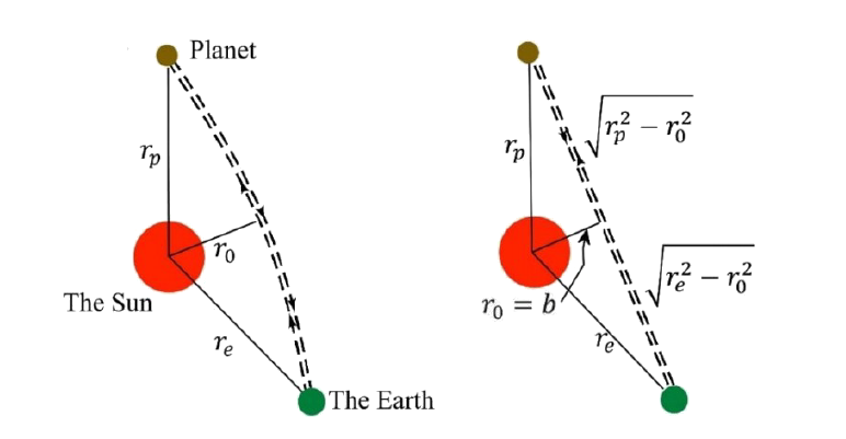
In the Shapiro experiment, radar signals were sent from Earth to a planet that was located on the opposite side of the Sun at that time. These signals were reflected back to Earth. According to general relativity, the signal, which passes close to the Sun, is deflected by the Sun’s gravitational field, or more precisely, the mass of the Sun warps spacetime such that the signal follows a “straight curved” trajectory.

vector_4_5_5
Figure 1: Radar reflection of photons from Earth to a planet and back. The left image shows the actual path, exaggerated. The right image shows the Euclidean form.
(From Tests of General Relativity: A Review by Estelle Asmodelle (Asmodelle, 2017))

To define the Shapiro delay, we assume that the Earth and the planet are stationary, while the total time for the round trip of the radar signal is \( \Delta t \), in coordinate time. The value of \( t \) must be expressed in terms of \( r \) over the entire path, where \( r_0 \) is the closest distance to the Sun.

4.5.1 Derivation based on the Schwarzschild metric

For the calculation of the Shapiro delay, the Schwarzschild equation is applied:

\begin{align} ds^{2} = c^{2} d\tau^{2} = \sigma^{2} c^{2} dt^{2} - \frac{dr^{2}}{\sigma^{2}} - r^{2} d\theta^{2} - r^{2}\sin^{2}\theta \, d\phi^{2} \label{eq:R409} \end{align}

Where:

\begin{align} \sigma =\sqrt{ 1 - \frac{2GM_{\text{sun}}}{c^{2} r}} = \sqrt{1 - \frac{R_{s}}{r}} \label{eq:R410} \end{align}

and

\begin{align} R_{s} = \frac{2GM_{\text{sun}}}{c^{2}} \label{eq:R411} \end{align}
the Schwarzschild radius of the Sun.

We choose the reference frame such that it coincides with the equatorial plane, (\( \theta = \pi/2 \) )

Then we have:

\begin{align} c^2 d\tau^2 = \sigma^2 c^2 dt^2 - \frac{dr^2}{\sigma^2} - r^2 d\phi^2 \label{eq:R412} \end{align}

For photons or radar echoes we have \(d\tau = 0\), hence:

\begin{align} \sigma^2 c^2 dt^2 = \frac{dr^2}{\sigma^2} + r^2 d\phi^2 \label{eq:R413} \end{align}

Differentiation with respect to the affine parameter \(\lambda\):

\begin{align} \sigma^2 c^2 \left(\frac{dt}{d\lambda}\right)^2 = \frac{1}{\sigma^2} \left(\frac{dr}{d\lambda}\right)^2 + r^2 \left(\frac{d\phi}{d\lambda}\right)^2 \label{eq:R414} \end{align}

As derived in equation (\ref{eq:R131}) from chapter 4.2, the angular momentum is:

\begin{align} L = r^2 \frac{d\phi}{d\lambda} \label{eq:R415} \end{align}
and
\begin{align}\sigma^2 c^2 \left(\frac{dt}{d\lambda}\right)^2 = \frac{1}{\sigma^2} \left(\frac{dr}{d\lambda}\right)^2 + \frac{L^2}{r^2} \label{eq:R416} \end{align}

Multiply by \(\sigma^2\):

\begin{align} \sigma^4 c^2 \left(\frac{dt}{d\lambda}\right)^2 = \left(\frac{dr}{d\lambda}\right)^2 + \frac{L^2}{r^2} \sigma^2 \label{eq:R417} \end{align}

Define:

\begin{align} k^2 = \sigma^4 \left(\frac{dt}{d\lambda}\right)^2 \label{eq:R418} \end{align}
Note: This is also \(k = E /c^2\) as seen in equation (\ref{eq:R127}) from chapter 4.2.
Then:

\begin{align}\left(\frac{dr}{d\lambda}\right)^2 + \frac{L^2}{r^2} \sigma^2 = k^2 c^2\label{eq:R419} \end{align}
The energy equation for a photon trajectory in the Schwarzschild geometry is therefore:
\begin{align} \left(\frac{dr}{d\lambda}\right)^2 + \frac{L^2}{r^2} \left(1 - \frac{R_s}{r}\right) = k^2 c^2 \label{eq:R420} \end{align}

As previously derived:

\begin{align} k^2 = \sigma^4 \left(\frac{dt}{d\lambda}\right)^2 \Rightarrow \left(\frac{dt}{d\lambda}\right)^2 = \frac{k^2}{\sigma^4} \label{eq:R421} \end{align}

Where we use:

\begin{align} \left(\frac{dt}{d\lambda}\right)^2 = \frac{k^2}{\sigma^4} = \frac{k^2}{(1-R_s/r)^2} \label{eq:R422} \end{align}

Now:

\begin{align} \left(\frac{dr}{d\lambda}\right)^2 = \left(\frac{dr}{dt} \frac{dt}{d\lambda}\right)^2 = \frac{k^2}{(1-R_s/r)^2} \left(\frac{dr}{dt}\right)^2 \label{eq:R423} \end{align}

We can rewrite the energy equation (\ref{eq:R420}):

\begin{align} \left(\frac{dr}{d\lambda}\right)^2 +\frac{L^2}{r^2}\left(1-\frac{R_s}{r}\right)=k^2c^2 \label{eq:R424} \end{align}
Substitute \(\left(\frac{dr}{d\lambda}\right)^2 \) using ((\ref{eq:R421}):
\begin{align} \frac{k^2}{(1-R_s/r)^2} \left(\frac{dr}{dt}\right)^2 + \frac{L^2}{r^2} (1-R_s/r) = k^2 c^2 \label{eq:R425} \end{align}
Divide by \((1-R_s/r)\):
\begin{align} \frac{k^2}{(1-R_s/r)^3} \left(\frac{dr}{dt}\right)^2 + \frac{L^2}{r^2} - \frac{k^2 c^2}{1-R_s/r} = 0 \label{eq:R426} \end{align}

Next, divide by \(k^2\):

\begin{align} \frac{1}{(1-R_s/r)^3} \left(\frac{dr}{dt}\right)^2 + \frac{L^2}{k^2r^2} - \frac{c^2}{1-R_s/r} = 0 \label{eq:R427} \end{align}
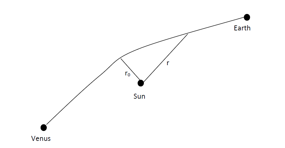
Now consider the path of a photon from Earth to another planet (for example Venus, with \(r_p=r_v\)), as shown in Figure 2. It is clear that the photon’s path will be deflected by the Sun’s gravitational field. Let \(r_0\) be the coordinate distance of the closest approach of the photon to the Sun; then:
\begin{align} \left(\frac{dr}{dt}\right)_{r_0}=0 \label{eq:R428} \end{align}
Then from (43) we find the relation between the constants:
\begin{align} \frac{L^2}{k^2r^2} = \frac{c^2}{1-R_s/r} \label{eq:R429} \end{align}
After rearranging, we can write (\ref{eq:R427}) as:
\begin{align} \left(\frac{dr}{dt}\right)^2 =\left(1-R_s/r\right)^3\left(-\frac{L^2}{k^2r^2} + \frac{c^2}{1-R_s/r}\right) =\left(1-R_s/r\right)^3\left(\frac{c^2}{1-R_s/r}-\frac{L^2r_0^2}{k^2r_0^2r^2}\right) \label{eq:R430} \end{align}

\begin{align} =\left(1-R_s/r\right)^3\left(\frac{c^2}{1-R_s/r}-\frac{r_0^2 c^2}{r^2\left(1-R_s/r_0\right)}\right) \label{eq:R431} \end{align}

\begin{align} =\left(1-R_s/r\right)^2\left(c^2-\frac{r_0^2c^2(1-R_s/r)}{r^2(1-R_s/r_0)}\right) =c^2\left(1-R_s/r\right)^2\left(1-\frac{r_0^2(1-R_s/r)}{r^2(1-R_s/r_0)}\right) \label{eq:R432} \end{align}
\begin{align} \Rightarrow \frac{dr}{dt}=c\left(1-R_s/r\right)\left[1-\frac{r_0^2(1-R_s/r)}{r^2(1-R_s/r_0)}\right]^{1/2} \label{eq:R433} \end{align}

vector_4_5_1_1
Figure 2 Photon path from Earth to Venus, deflected by the Sun.

This can be integrated to determine the time required to travel between the point \(r_0\) and \(r\):

\begin{align} t(r,r_0)=\int_{r_0}^{r} \frac{1}{c\left(1-R_s/r\right)\left[1-\frac{r_0^2(1-R_s/r)}{r^2(1-R_s/r_0)} \right]^{1/2}}\,dr \label{eq:R434} \end{align}

4.5.1.1 First-order approximation

Since \(R_{s} \ll r_{0}\), we can take the first-order Taylor approximation of:

\begin{align} \frac{1 - \frac{R_{s}}{r}}{1 - \frac{R_{s}}{r_{0}}} \approx \left(1 - \frac{R_{s}}{r}\right) \left(1 + \frac{R_{s}}{r_{0}}\right) = 1 - \frac{R_{s}}{r} + \frac{R_{s}}{r_{0}} - \frac{R_{s}^{2}}{rr_{0}} \label{eq:R435} \end{align}

Thus, the integrand can be expanded to first order in \(R_{s}/r\):

\begin{align} t(r,r_{0}) =\int_{r_0}^r \frac{1}{c(1-R_s/r)\left[1-\frac{r_0^2}{r^2} \left(1-\frac{R_s}{r}+\frac{R_s}{r_0}-\frac{R_s^2}{rr_0}\right)\right]^{1/2}}\, dr \label{eq:R436} \end{align}

Multiply the numerator and denominator by \(r\):

\begin{align} t(r,r_{0}) =\int_{r_0}^r \frac{r}{c(1-R_s/r)\left[r^2-r_0^2 \left(1-\frac{R_s}{r}+\frac{R_s}{r_0}-\frac{R_s^2}{rr_0}\right)\right]^{1/2}}\, dr \label{eq:R437} \end{align}
\begin{align} t(r,r_{0}) =\int_{r_0}^r \frac{r}{c(1-R_s/r)\left[r^2-r_0^2-R_sr_0 +\frac{R_sr_0^2}{r}+\frac{R_s^2r_0}{r}\right]^{1/2}}\, dr \label{eq:R438} \end{align}
\begin{align} t(r,r_{0}) =\int_{r_0}^r \frac{r}{c\sqrt{r^2-r_0^2}(1-R_s/r)\left[1- \frac{R_sr_0\left(1-\frac{r_0}{r}-\frac{R_s}{r}\right)}{r^2-r_0^2}\right]^{1/2}}\, dr \label{eq:R439} \end{align}
\begin{align} t(r,r_{0}) =\int_{r_0}^r \frac{r}{c\sqrt{r^2-r_0^2}\left[\left(1-\frac{2R_s}{r}+\frac{R_s^2}{r^2}\right)\left(1- \frac{R_sr_0\left(1-\frac{r_0}{r}-\frac{R_s}{r}\right)}{r^2-r_0^2}\right)\right]^{1/2}}\, dr \label{eq:R440} \end{align}

First, we expand the right-hand side of the numerator:

\begin{align} \left(1-\frac{2R_s}{r}+\frac{R_s^2}{r^2}\right)\left(1- \frac{R_sr_0\left(1-\frac{r_0}{r}-\frac{R_s}{r}\right)}{r^2-r_0^2}\right) \label{eq:R441} \end{align}
\begin{align} 1-\frac{2R_s}{r}+\frac{R_s^2}{r^2}-\frac{R_sr_0\left(1-\frac{r_0}{r}-\frac{R_s}{r}\right)}{r^2-r_0^2} +\frac{2R_s^2r_0\left(1-\frac{r_0}{r}-\frac{R_s}{r}\right)}{r(r^2-r_0^2)} -\frac{R_s^3r_0\left(1-\frac{r_0}{r}-\frac{R_s}{r}\right)}{r^2(r^2-r_0^2)} \label{eq:R442} \end{align}

After neglecting the smallest terms:

\begin{align} \left(1-\frac{2R_s}{r}+\frac{R_s^2}{r^2}\right)\left(1- \frac{R_sr_0\left(1-\frac{r_0}{r}-\frac{R_s}{r}\right)}{r^2-r_0^2}\right) \approx 1-\frac{2R_s}{r}-\frac{R_sr_0\left(1-\frac{r_0}{r}\right)}{r^2-r_0^2} \label{eq:R443} \end{align}
\begin{align} \left(1-\frac{2R_s}{r}+\frac{R_s^2}{r^2}\right)\left(1- \frac{R_sr_0\left(1-\frac{r_0}{r}-\frac{R_s}{r}\right)}{r^2-r_0^2}\right) \approx 1-\frac{2R_s}{r}-\frac{R_sr_0\left(r-r_0\right)}{r(r+r_0)(r-r_0)} \label{eq:R444} \end{align}
\begin{align} \left(1-\frac{2R_s}{r}+\frac{R_s^2}{r^2}\right)\left(1- \frac{R_sr_0\left(1-\frac{r_0}{r}-\frac{R_s}{r}\right)}{r^2-r_0^2}\right) \approx 1-\frac{2R_s}{r}-\frac{R_sr_0}{r(r+r_0)} \label{eq:R445} \end{align}

Substitute into the denominator:

\begin{align} t(r,r_{0}) =\int_{r_0}^r \frac{r}{c\sqrt{r^2-r_0^2}\left[1-\frac{2R_s}{r}-\frac{R_sr_0}{r(r+r_0)}\right]^{1/2}}\, dr \label{eq:R446} \end{align}

Applying again a first-order Taylor approximation, we obtain:

\begin{align} t(r,r_{0}) =\int_{r_0}^r \frac{r}{c\sqrt{r^2-r_0^2}}\left[1+\frac{R_s}{r}+\frac{R_sr_0}{2r(r+r_0)}\right]\, dr \label{eq:R447} \end{align}

This can be reduced to (see verification below):

\begin{align} t(r,r_{0}) = \frac{\sqrt{r^{2}-r_{0}^{2}}}{c} + \frac{R_{s}}{c} \ln\!\left(\frac{ r + \sqrt{r^{2}-r_{0}^{2}}}{r_0} \right) + \frac{R_{s}}{2c} \left(\frac{r - r_{0}}{r + r_{0}}\right)^{1/2} \label{eq:R448} \end{align}

Verification of the above formula

We can verify the above formula by taking the derivative; this must equal the integrand:

\begin{align} \frac{dt(r,r_0)}{dr}=\frac{r}{c(r^2-r_0^2)^{1/2}}+ \frac{R_s}{c} \frac{\left( \frac{1}{r_0}+\frac{r}{r_0(r^2-r_0^2)^{1/2}}\right)}{\frac{r+(r^2-r_0^2){1/2}}{r_0}} +\frac{R_s}{4c}\frac{\left(\frac{1}{r+r_0}-\frac{r-r_0}{(r+r_0)^{2}} \right)}{\left( \frac{r-r_0}{r+r_0}\right)^{1/2}} \label{eq:R449} \end{align}
\begin{align} \frac{dt(r,r_0)}{dr}=\frac{r}{c(r^2-r_0^2)^{1/2}}+ \frac{R_s}{c} \frac{\left( 1+\frac{r}{(r^2-r_0^2)^{1/2}}\right)}{r+(r^2-r_0^2){1/2}} +\frac{R_s}{4c}\frac{\left(\frac{r+r_0-r+r_0}{(r+r_0)^{2}} \right)} {\left( \frac{r-r_0}{r+r_0}\right)^{1/2}} \label{eq:R450} \end{align}
\begin{align} \frac{dt(r,r_0)}{dr}=\frac{r}{c(r^2-r_0^2)^{1/2}}+ \frac{R_s}{c} \frac{\left[ r+(r^2-r_0^2)^{1/2}\right]}{\left[r+(r^2-r_0^2)^{1/2}\right](r^2-r_0^2)^{1/2}} +\frac{R_s}{4c} \frac{\left(r+r_0-r+r_0\right)} {\left( \frac{r-r_0}{r+r_0}\right)^{1/2}(r+r_0)^{2}} \label{eq:R451} \end{align}
\begin{align} \frac{dt(r,r_0)}{dr}=\frac{r}{c(r^2-r_0^2)^{1/2}}+ \frac{R_s}{c} \frac{1}{(r^2-r_0^2)^{1/2}} +\frac{R_s}{2c} \frac{r_0} {\left( \frac{r-r_0}{r+r_0}\right)^{1/2}(r+r_0)^{2}} \label{eq:R452} \end{align}
\begin{align} \frac{dt(r,r_0)}{dr}=\frac{r}{c(r^2-r_0^2)^{1/2}}+ \frac{R_s}{c} \frac{1}{(r^2-r_0^2)^{1/2}} +\frac{R_s}{2c} \frac{r_0} {(r-r_0)^{1/2}(r+r_0)} \label{eq:R453} \end{align}
\begin{align} \frac{dt(r,r_0)}{dr}=\frac{r}{c(r^2-r_0^2)^{1/2}} \left[ 1+ \frac{R_s}{r}+\frac{R_sr_0}{2r(r+r_0)} \right] \label{eq:R454} \end{align}

Thus, the formula is correct!


Therefore:

\begin{align} t(r,r_{0}) = \frac{\sqrt{r^{2}-r_{0}^{2}}}{c} + \frac{R_{s}}{c} \ln\!\left(\frac{ r + \sqrt{r^{2}-r_{0}^{2}}}{r_0} \right) + \frac{R_{s}}{2c} \left(\frac{r - r_{0}}{r + r_{0}}\right)^{1/2} \label{eq:R455} \end{align}

The first term on the right-hand side is exactly what we would expect if light traveled in a straight line. The second and third terms represent the additional coordinate time required for the photon to travel along the curved path to the point \(r\).

As shown in Figure 2, if we send a radar signal to Venus and back, then the extra coordinate time relative to a straight-line path is:

\begin{align} \Delta t = 2\left[ t(r_{E},r_{0}) + t(r_{V},r_{0}) - \frac{\sqrt{r_{E}^{2}-r_{0}^{2}}}{c} - \frac{\sqrt{r_{V}^{2}-r_{0}^{2}}}{c} \right] \label{eq:R456} \end{align}

As mentioned earlier, the first two terms inside the brackets represent the relativistic time from Earth to Venus, and the two terms on the right represent the time if the path were simply a straight line. The factor 2 is included because the photon must travel to Venus and back to Earth.

Since \(r_{E} \gg r_{0}\) and \(r_{V} \gg r_{0}\), we have:

\begin{align} t(r_{E},r_{0}) - \frac{\sqrt{r_{E}^{2}-r_{0}^{2}}}{c} \approx \frac{R_{s}}{c} \ln\!\left( \frac{r_{E} + r_{E}}{r_{0}} \right) + \frac{R_{s}}{2c} = \frac{R_{s}}{c} \ln\!\left( \frac{2r_{E}}{r_{0}} \right) + \frac{R_{s}}{2c} \label{eq:R457} \end{align}
\begin{align} t(r_{V},r_{0}) - \frac{\sqrt{r_{V}^{2}-r_{0}^{2}}}{c} \approx \frac{R_{s}}{c} \ln\!\left( \frac{r_{V} + r_{V}}{r_{0}} \right) + \frac{R_{s}}{2c} = \frac{R_{s}}{c} \ln\!\left( \frac{2r_{V}}{r_{0}} \right) + \frac{R_{s}}{2c} \label{eq:R458} \end{align}

Summation:

\begin{align} \frac{R_{s}}{c} \ln\!\left(\frac{2r_{E}}{r_{0}}\right) + \frac{R_{s}}{c} \ln\!\left(\frac{2r_{V}}{r_{0}}\right) + \frac{R_{s}}{c} = \frac{2GM}{c^{3}} \left[ \ln\!\left( \frac{4 r_{E} r_{V}}{r_{0}^{2}} \right) + 1 \right] \label{eq:R459} \end{align}

Thus, for a round trip to Venus, the additional coordinate time delay is:

\begin{align} \Delta t \approx \frac{4GM_{\text{sun}}}{c^{3}} \left[ \ln\!\left( \frac{4 r_{E} r_{V}}{r_{0}^{2}} \right) + 1 \right] \label{eq:R460} \end{align}

This also shows that the time delay increases as the impact parameter \(r_{0}\) (the distance to the gravitational center) decreases.

Numerical Values

  • For Venus, opposite Earth on the far side of the Sun: \(\Delta t ≈ 252\, μs\)
  • For Mercury: \(\Delta t ≈ 240\, μs\)
  • Distance Venus–Sun \(r_V : 108 × 10^9 \,m\)
  • Distance Sun–Earth \(r_E : 150 × 10^9 \,m\)
  • Total distance Venus–Earth: \(258 × 10^9 \,m\)
  • Total travel time (Earth → Sun → Venus → Earth) without delay: \(1720\, s\)

The Shapiro delay is therefore small, but clearly measurable.

4.5.1.2 Proper time on Earth versus coordinate time

Clocks on Earth do not measure coordinate time, due to the rotation of the Earth about its own axis and the effect of Earth's orbital motion around the Sun.
Due to the rotation of the Earth about its own axis, the corresponding proper time of the signal is given by:

\begin{align}\Delta \tau = \sqrt{1 - \frac{2 G M_E}{c^2 r_E}} \, \Delta t\label{eq:R461} \end{align}

The effect is therefore:

\begin{align} \Delta t -\Delta \tau =\Delta t - \sqrt{1 - \frac{2 G M_E}{c^2 r_E}} \, \Delta t \label{eq:R462} \end{align}
This gives:
\begin{align} \Rightarrow 6.98*10^{-10} \Delta t \,\, for \,\, 252 \, \mu s \Rightarrow 1.76* 10^{-13} seconds=0.176\,ps \label{eq:R463} \end{align}
\begin{align} p=10^{-12} \label{eq:R464} \end{align}

Since \(r_E\,\gg\, GM/c^2\), and thus \(0.176\,ps \,\ll \,252\, \mu s\), this effect is negligible.

The effect of Earth's orbital motion around the Sun causes a delay of 15 nanoseconds per second, as mentioned in chapter 4.6.
For the additional time delay \( \Delta t \approx 252\, \mu s\) from Venus, Earth's orbital motion around the Sun produces a small effect of: \(252∗10^{−6}∗15∗10^{-9}=3.78∗10^{−12}\, seconds=3.78\, ps\), which can also be neglected.

4.5.2 Physical Interpretation

  • The additional time delay is a direct consequence of the curvature of spacetime caused by the Sun.
  • The effect is largest when the signal passes close to the Sun (small \(r_0\)).
  • Experiments show that the measured time delay exactly matches the predictions of general relativity.

4.5.3 Practical significance

  • Important for precise navigation of space missions and for testing alternative theories of gravity.
  • Used in pulsar timing and in interpreting signals from spacecraft.

4.5.4 Key insight

The Shapiro time delay is one of the four classical experiments that confirm general relativity. The effect is small, but measurable and fully explained by the Schwarzschild metric.

4.6 Time relation between an observer on Earth and the center of the Sun

When considering the deflection of light or the motion of planets around the Sun, a reference frame is used with its origin at the center of the Sun, while we observe the phenomenon from Earth and have a rotational velocity relative to the Sun. In this chapter, we investigate the time relation between an observer on Earth and the center of the Sun, including the corresponding correction factors.

The starting point is the Schwarzschild metric, which describes spacetime around a spherically symmetric massive object. The metric is given by:

\begin{align} ds^2 = \sigma^2 c^2 dt^2 - \frac{dr^2}{\sigma^2} - r^2 d\theta^2 - r^2 \sin^2\theta \, d\phi^2 \label{eq:R465} \end{align}

where:

\begin{align} \sigma =\sqrt{ 1 - \frac{2 G M_{\text{sun}}}{c^2 r}}, \qquad R_s = \frac{2 G M_{\text{sun}}}{c^2} \label{eq:R466} \end{align}
  • G is the gravitational constant,
  • Msun is the mass of the Sun,
  • c is the speed of light,
  • R is the distance to the center of the Sun.

The coordinates \(\theta\) and \(\phi\) represent the usual spherical coordinates. We restrict ourselves to the equatorial plane of the Sun, so that \(\theta\, =\, \pi /2\) and the radius \(r\) is constant.

4.6.1 Simplification of the Schwarzschild metric

For an observer on Earth, we assume that Earth moves in a circular orbit around the Sun. The time measurement of the observer on Earth is described by the proper time , while dt is the coordinate time in the Sun reference frame.

The Schwarzschild metric then reduces to:

\begin{align} ds^2 = c^2 d\tau^2 = \sigma^2 c^2 dt^2 - r^2 d\phi^2 \label{eq:R467} \end{align}

This can be rewritten as:

\begin{align} d\tau^2 = \sigma^2 dt^2 - \frac{r^2}{c^2} \left( \frac{d\phi}{dt} \right)^2 dt^2 \label{eq:R468} \end{align}

Substituting \(\sigma\) gives:

\begin{align} d\tau^2 = \left( 1 - \frac{R_s}{r} - \frac{r^2}{c^2} \left( \frac{d\phi}{dt} \right)^2 \right) dt^2 \label{eq:R469} \end{align}

4.6.2 Time dilation due to gravity and motion of the Earth

For an observer on Earth:

\begin{align} d\tau^2 = \left( 1 - \frac{R_s}{r} - \frac{v^2}{c^2} \right) dt^2 \label{eq:R470} \end{align}
\begin{align} d\tau = \sqrt{ 1 - \frac{R_s}{r} - \frac{v^2}{c^2} } \, dt \label{eq:R471} \end{align}

where \(R_s\) is the Schwarzschild radius of the Sun, \(v\) is the orbital velocity of Earth, and \(r\) is the distance from Earth to the center of the Sun. This is the general time relation that accounts for both the Sun’s gravitational field and Earth’s velocity.

Numerical values:

  • \( R_s = 2950 \,\text{m} \)
  • \( v =30.000 \,\text{m/s} \)
  • \( r = 150 \times 10^{9} \,\text{m (the average distance from Earth to the Sun).} \)

By substituting the values and expanding the expression for \(d\tau\) using a first-order Taylor series, we obtain the following approximation:

\begin{align} d\tau \approx \left( 1 - \frac{R_s}{2r} - \frac{v^2}{2c^2} \right) dt \label{eq:R472} \end{align}

The second term on the right-hand side is due to the gravitational field of the Sun, and the third term is due to Earth’s orbital velocity around the Sun.
Substituting the numerical values yields:

\begin{align} d\tau = \left( 1 - 9.9 \times 10^{-10} - 5.0 \times 10^{-9} \right) dt \label{eq:R473} \end{align}
\begin{align} d\tau \approx \left( 1 - 1.5 \times 10^{-8} \right) dt \label{eq:R474} \end{align}
\begin{align} \Delta t - \Delta \tau = 1.5 \times 10^{-8} \, \Delta t \label{eq:R475} \end{align}

This corresponds to a time delay of approximately 15 nanoseconds per second for an observer on Earth relative to Sun-centered coordinate time.

4.6.3 Correction factor for Earth's gravity

An observer on Earth is also affected by Earth's gravitational field. This effect must also be taken into account for a complete description of the time relation. The proper time \( d\tau \) is in this case modified by Earth's gravity, using the following metric:

\begin{align} d\tau = \sqrt{ 1 - \frac{2 G M_E}{c^2 r_E} } \, dt \label{eq:R476} \end{align}

With:

  • \( M_E = 5.9742 \times 10^{24} \,\text{kg}\,\text{(mass of the Earth)} \)
  • \( r_E = 6.381 \times 10^{6} \,\text{m}\, \text{(radius of the Earth)}\)

This gives:

\begin{align} d\tau=\sqrt{1-1.3908*10^{-9}}dt \approx \left( 1 - 0.6954 \times 10^{-9} \right) dt \label{eq:R477} \end{align}

For an observer at the equator, the rotational velocity \(v_{rot}\) of the Earth is also relevant. The angular velocity \(d\phi/dt\) of the Earth is given by its rotation period (sidereal period: \(86162.4 \text{ seconds}\)):

\begin{align} \frac{d\phi}{dt} = \frac{2\pi}{T_{tot}} = \frac{2\pi}{86162.4} = 7.2923 \times 10^{-5} \,\text{rad/s} \label{eq:R478} \end{align}

The modified time relation for an observer at the equator, including Earth's rotation, is then:

\begin{align} d\tau=\sqrt{\left(1-\frac{R_E}{r^e}-\frac{v_E^2}{c^2}\right)}\,dt \label{eq:R479} \end{align}

where the second term represents the contribution from Earth's rotational velocity. Substituting the appropriate values yields the final time relation:

\begin{align} d\tau = \sqrt{ 1 - 1.3908 \times 10^{-9} - 2.4059 \times 10^{-12}} dt \label{eq:R480} \end{align}
\begin{align} d\tau \approx \left( 1 - 0.6966 \times 10^{-9} \right) dt \label{eq:R481} \end{align}

Where:

  • \( R_E = 0.008875 \,\text{m} \) (Schwarzschild radius of the Earth)
  • \( r_e = 6{,}381{,}000 \,\text{m} \) (radius of the Earth)
  • \( v_E = 465 \,\text{m/s} \) (rotation of the Earth about its axis)
  • \( c = 3 \cdot 10^{8} \,\text{m/s} \)

4.6.4 Conclusion

The time relation between an observer on Earth and the center of the Sun is determined by three effects: the Sun’s gravitational field, Earth's orbital velocity, and the local gravitational field of the Earth itself. Together, they produce a small but measurable time delay.

4.6.5 Physical interpretation

  • Clocks on Earth run slower than a hypothetical clock at the center of the Sun.
  • These corrections are essential for GPS, space navigation, and precision timing.

4.7 Alternative derivation of the orbit equation

According to Kepler’s first law, all planetary orbits around the Sun are elliptical. As we saw in chapter 4.4, general relativity shows that there is also a relativistic correction to this elliptical shape, which explains the perihelion precession of, for example, Mercury.

We therefore present here an alternative derivation of the orbit equation for a massive particle in Schwarzschild geometry that yields a solution closer to the original ellipse formula.

This is:

\begin{align} r(\phi) = a\,\frac{1 - e^{2}}{1 + e \cos(\phi - \theta)} \label{eq:R482} \end{align}

This equation is compared with the relativistic result (see equation (\ref{eq:R539}) at the end of this chapter:

\begin{align} r = a\,\frac{1 - e^{2}}{1 + e \cos(\phi - \epsilon \phi)} \label{eq:R483} \end{align}

Here we see that \( \theta \) is not a constant but a function of \( \phi \) and varies with a factor \( \epsilon \).

From General Relativity: An Introduction for Physics by M. P. Hobson, G. Efstathiou and A. N. Lasenby, p. 230 (Hobson, 2006).

We restrict ourselves to the equatorial plane \( \theta = \pi/2 \), so that the Schwarzschild metric for a massive particle reduces to:

\begin{align} c^{2} d\tau^{2} = c^{2}\left(1 - \frac{2GM}{c^{2} r}\right) dt^{2} - \left(1 - \frac{2GM}{c^{2} r}\right)^{-1} dr^{2} - r^{2} d\phi^{2} \label{eq:R484} \end{align}

The metric equation then becomes:

\begin{align} c^{2}\left(1 - \frac{2GM}{c^{2} r}\right) \left(\frac{dt}{d\tau}\right)^{2} - \left(1 - \frac{2GM}{c^{2} r}\right)^{-1} \left(\frac{dr}{d\tau}\right)^{2} - r^{2}\left(\frac{d\phi}{d\tau}\right)^{2} = c^{2} \label{eq:R485} \end{align}

After multiplying by \( 1 - \frac{2GM}{c^{2} r} \):

\begin{align} c^{2}\left(1 - \frac{2GM}{c^{2} r}\right)^{2} \left(\frac{dt}{d\tau}\right)^{2} - \left(\frac{dr}{d\tau}\right)^{2} - r^{2}\left(\frac{d\phi}{d\tau}\right)^{2} \left(1 - \frac{2GM}{c^{2} r}\right) = c^{2}\left(1 - \frac{2GM}{c^{2} r}\right) \label{eq:R486} \end{align}

Rearranging:

\begin{align} \left(\frac{dr}{d\tau}\right)^{2} + r^{2}\left(\frac{d\phi}{d\tau}\right)^{2} \left(1 - \frac{2GM}{c^{2} r}\right) - c^{2}\left(1 - \frac{2GM}{c^{2} r}\right)^{2} \left(\frac{dt}{d\tau}\right)^{2} = c^{2}\left(\frac{2GM}{c^{2} r} - 1\right) \label{eq:R487} \end{align}

We substitute the conserved quantities:

\begin{align} \left(1 - \frac{2GM}{c^{2} r}\right)\frac{dt}{d\tau} = \frac{E}{c^{2}}, \qquad r^{2}\frac{d\phi}{d\tau} = L \label{eq:R488} \end{align}

We then obtain:

\begin{align} \left(\frac{dr}{d\tau}\right)^{2} + \frac{L^{2}}{r^{2}}\left(1 - \frac{2GM}{c^{2} r}\right) - \frac{E^{2}}{c^{2}} = c^{2}\left(\frac{2GM}{c^{2} r} - 1\right) = \frac{2GM}{r} - c^{2} \label{eq:R489} \end{align}

\begin{align} \left(\frac{dr}{d\tau}\right)^{2} + \frac{L^{2}}{r^{2}}\left(1 - \frac{2GM}{c^{2} r}\right) - \frac{2GM}{r} = c^{2}\left(\frac{E^{2}}{c^{4}} - 1\right) \label{eq:R490} \end{align}

\begin{align} \left(\frac{dr}{d\tau}\right)^{2} + \frac{L^{2}}{r^{2}} = c^{2}\left(\frac{E^{2}}{c^{4}} - 1\right) + \frac{2GM}{r} + \frac{2GM L^{2}}{c^{2} r^{3}} \label{eq:R491} \end{align}

Now:

\begin{align} \frac{dr}{d\tau} = \frac{dr}{d\phi}\frac{d\phi}{d\tau} = \frac{L}{r^{2}}\frac{dr}{d\phi} \label{eq:R492} \end{align}

This substituted into the previous equation:

\begin{align} \left(\frac{L}{r^{2}}\frac{dr}{d\phi}\right)^{2} + \frac{L}{r^{2}} = c^{2}\left(\frac{E^{2}}{c^{4}} - 1\right) + 2GM r + \frac{2GM L^{2}}{c^{2} r^{3}} \label{eq:R493} \end{align}

Divide by \(L^{2}\):

\begin{align} \left(\frac{1}{r^{2}}\frac{dr}{d\phi}\right)^{2} + \frac{1}{r^{2}} = \frac{c^{2}}{L^{2}}\left(\frac{E^{2}}{c^{4}} - 1\right) + \frac{2GM}{L^{2} r} + \frac{2GM}{c^{2} r^{3}} \label{eq:R494} \end{align}

Now substitute \(u = 1/r\):

\begin{align} \frac{du}{d\phi} = \frac{du}{dr}\frac{dr}{d\phi} = -\frac{1}{r^{2}}\frac{dr}{d\phi} \quad\Rightarrow\quad \frac{1}{r^{2}}\frac{dr}{d\phi} = -\frac{du}{d\phi} \label{eq:R495} \end{align}

The equation now becomes:

\begin{align} \left(\frac{du}{d\phi}\right)^{2} + u^{2} = \frac{c^{2}}{L^{2}}\left(\frac{E^{2}}{c^{4}} - 1\right) + \frac{2GM}{L^{2}}u + \frac{2GM}{c^{2}}u^{3} \label{eq:R496} \end{align}

We differentiate this equation with respect to \( \phi \) to obtain:

\begin{align} 2\frac{du}{d\phi}\frac{d^{2}u}{d\phi^{2}} + 2u\frac{du}{d\phi} = \frac{2GM}{L^{2}}\frac{du}{d\phi} + 6\frac{GM}{c^{2}}u^{2}\frac{du}{d\phi} \label{eq:R497} \end{align}

We divide by \(2\,\frac{du}{d\phi}\) (assuming that \(\frac{du}{d\phi} \neq 0\)):

\begin{align} \frac{d^{2}u}{d\phi^{2}} + u = \frac{GM}{L^{2}} + \frac{3GM}{c^{2}}u^{2} \label{eq:R498} \end{align}

If we temporarily neglect the last term, we obtain the equation according to Newtonian theory, whose solution is:

\begin{align} u = \frac{GM}{L^{2}}\left(1 + e\cos\phi\right) \quad\text{or}\quad r = \frac{L^{2}}{GM}\,\frac{1}{1 + e\cos\phi} \label{eq:R499} \end{align}

This describes an ellipse, where the parameter \(e\) represents the eccentricity of the orbit. For example, we can describe the orbit of a planet around the Sun. We can write the distance to the closest point (perihelion) as:

\begin{align} r_{1} = a(1 - e) \label{eq:R500} \end{align}
and the distance to the farthest point (aphelion) as:
\begin{align} r_{2} = a(1 + e). \label{eq:R501} \end{align}

Derived from (\ref{eq:R499}) and again substituting \( r = 1/u \) gives:

\begin{align} r = \frac{L^{2}}{GM}\,\frac{1}{1 + e\cos\phi} \quad\Rightarrow\quad r_{\max} = \frac{L^{2}}{GM}\,\frac{1}{1 - e}, \qquad r_{\min} = \frac{L^{2}}{GM}\,\frac{1}{1 + e}. \label{eq:R502} \end{align}

The semi-major axis \(a\) is then given by:

\begin{align} a = \frac{r_{\max} + r_{\min}}{2} = \frac{L^{2}}{2GM} \left( \frac{1}{1 - e} + \frac{1}{1 + e} \right) = \frac{L^{2}}{2GM} \left( \frac{1 + e + 1 - e}{1 - e^{2}} \right) \label{eq:R503} \end{align}

Thus, the equation of motion requires that the semi-major axis is given by:

\begin{align} a = \frac{L^{2}}{GM}\,\frac{1}{1 - e^{2}} \label{eq:R504} \end{align}

Thus:

\begin{align} r_{\max} = \frac{L^{2}}{GM}\,\frac{1}{1 - e} = a(1 + e), \qquad r_{\min} = \frac{L^{2}}{GM}\,\frac{1}{1 + e} = a(1 - e). \label{eq:R505} \end{align}

vector_4_7_1
Elliptical orbit of a planet around the Sun; e is the eccentricity of the orbit.

Now, to include the third term (from equation (\ref{eq:R498})), the solution becomes:

\begin{align} u = \frac{GM}{L^{2}}\left(1 + e\cos\phi\right) + \Delta u \label{eq:R506} \end{align}

\begin{align} \frac{du}{d\phi} = -\frac{GM}{L^{2}}\,e\sin\phi + \frac{d\Delta u}{d\phi}, \qquad \frac{d^{2}u}{d\phi^{2}} = -\frac{GM}{L^{2}}\,e\cos\phi + \frac{d^{2}\Delta u}{d\phi^{2}} \label{eq:R507} \end{align}

We substitute this into equation (\ref{eq:R498}):

\begin{align} \frac{d^{2}u}{d\phi^{2}} + u = \frac{GM}{L^{2}} + \frac{3GM}{c^{2}}u^{2} \label{eq:R508} \end{align}

\begin{align} \frac{d^{2}u}{d\phi^{2}} + u = \frac{GM}{L^{2}}\left(1 + e\cos\phi - e\cos\phi\right) + \frac{d^{2}\Delta u}{d\phi^{2}} + \Delta u = \frac{GM}{L^{2}} + \frac{d^{2}\Delta u}{d\phi^{2}} + \Delta u \label{eq:R509} \end{align}

\begin{align} \frac{d^{2}\Delta u}{d\phi^{2}} + \Delta u = -\frac{GM}{L^{2}} + \frac{d^{2}u}{d\phi^{2}} + u = -\frac{GM}{L^{2}} + \frac{GM}{L^{2}} + \frac{3GM}{c^{2}}u^{2} = \frac{3GM}{c^{2}}u^{2} \label{eq:R510} \end{align}

\begin{align} \begin{aligned} \frac{d^{2}\Delta u}{d\phi^{2}} + \Delta u &= \frac{3GM}{c^{2}} \left[ \left(\frac{GM}{L^{2}}\right)^{2} + \left(\frac{GM}{L^{2}} e\cos\phi\right)^2 +\left( \Delta u \right)^2 \right] \\ \notag &\quad + \frac{3GM}{c^{2}} \left[ 2\left(\frac{GM}{L^{2}}\right)^2 e\cos\phi + 2\frac{GM}{L^{2}}\Delta u + 2\frac{GM}{L^{2}} e\cos\phi\cdot\Delta u \right] \end{aligned} \label{eq:R511} \end{align}

We find that, to first order in \(\Delta u\):

\begin{align} \frac{d^{2}\Delta u}{d\phi^{2}} + \Delta u = \frac{3(GM)^3}{c^{2}L^{4}} \left[1 + \left(e\cos\phi\right)^{2}+2e \cos{\phi}\right] \label{eq:R512} \end{align}

A particular solution of the equation is:

\begin{align} \Delta u = \frac{3(GM)^3}{c^{2}L^{4}} \left[1+ e^{2}\left(\frac{1}{2} - \frac{1}{6}\cos(2\phi)\right) + e\phi\sin\phi \right] \label{eq:R513} \end{align}


This can be verified by direct differentiation of (\ref{eq:R513}):

\begin{align} \frac{d\Delta u}{d\phi} = \frac{3(GM)^3}{c^{2}L^{4}} \left[ \frac{1}{3}e^{2}\sin(2\phi) + e\sin\phi + e\phi\cos\phi \right] \label{eq:R514} \end{align}

\begin{align} \frac{d^{2}\Delta u}{d\phi^{2}} = \frac{3(GM)^3}{c^{2}L^{4}} \left[ \frac{2}{3}e^{2}\cos(2\phi) + e\cos\phi + e\cos\phi - e\phi\sin\phi \right] \label{eq:R515} \end{align}

\begin{align} \frac{d^{2}\Delta u}{d\phi^{2}} = \frac{3(GM)^3}{c^{2}L^{4}} \left[ \frac{2}{3}e^{2}\cos(2\phi) + 2e\cos\phi - e\phi\sin\phi \right] \label{eq:R516} \end{align}

Substituting into (\ref{eq:R513}):

\begin{align} \frac{d^{2}\Delta u}{d\phi^{2}} + \Delta u = \frac{3(GM)^3}{c^{2}L^{4}} \left[ \frac{2}{3}e^{2}\cos(2\phi) + 2e\cos\phi - e\phi\sin\phi+1+ e^2\left( \frac{1}{2}-\frac{1}{6}\cos(2\phi)\right) + e\phi\sin\phi \right] \label{eq:R517} \end{align}

\begin{align} \frac{d^{2}\Delta u}{d\phi^{2}} + \Delta u = \frac{3(GM)^3}{c^{2}L^{4}} \left(1 + \tfrac{1}{2}e^{2} + \tfrac{1}{2}e^{2}\cos 2\phi + 2e\cos\phi\right) \label{eq:R518} \end{align}

\begin{align} \frac{d^{2}\Delta u}{d\phi^{2}} + \Delta u = \frac{3(GM)^3}{c^{2}L^{4}} \left[1 + \frac{1}{2}e^{2}\left(1 + \cos 2\phi\right)+2e\cos\phi\right] \label{eq:R519} \end{align}

\begin{align} \frac{d^{2}\Delta u}{d\phi^{2}} + \Delta u = \frac{3(GM)^3}{c^{2}L^{4}} \left[ 1 + \frac{1}{2}e^{2}\left(\sin^{2}\phi + \cos^{2}\phi + \cos^{2}\phi - \sin^{2}\phi\right) + 2e\cos\phi \right] \label{eq:R520} \end{align}

\begin{align} \frac{d^{2}\Delta u}{d\phi^{2}} + \Delta u = \frac{3(GM)^3}{c^{2}L^{4}} \left(1 + e^{2}\cos^2\phi + 2e\cos\phi\right) \label{eq:R521} \end{align}

Thus, equation (\ref{eq:R498}) is correct.


Now we substitute \(\Delta u\) into equation (\ref{eq:R513}):

\begin{align} u = \frac{GM}{L^{2}}\left(1 + e\cos\phi\right) + \Delta u \label{eq:R522} \end{align}

\begin{align} u = \frac{GM}{L^{2}}\left(1 + e\cos\phi\right) + \frac{3(GM)^3}{c^{2}L^{4}} \left[1+e^{2}\left(\frac{1}{2}-\frac{1}{6}\cos{2\phi} \right)+e\phi\sin{\phi} \right] \label{eq:R523} \end{align}

\begin{align} u = \frac{GM}{L^{2}}\left(1 + e\cos\phi\right) + \frac{3(GM)^3}{c^{2}L^{4}}\,e\,\phi\sin\phi + \frac{3(GM)^3}{c^{2}L^{4}} \left[1 + e^{2}\left(\frac{1}{2} - \frac{1}{6}\cos 2\phi\right) \right] \label{eq:R524} \end{align}

Since the constant

\begin{align} \frac{3GM}{c^{2}L^{4}} \label{eq:R525} \end{align}
is very small, the last three terms on the right-hand side can be neglected — they are too small to have a measurable effect.

However, the last term

\begin{align} e\,\frac{3(GM)^3}{c^{2}L^{4}}\,\phi\sin\phi \label{eq:R526} \end{align}
is a special case: although small, it grows slowly with \(\phi\), since \(\phi\) itself keeps increasing. The effect accumulates and must therefore be retained.

\begin{align} u = \frac{GM}{L^{2}}\left[1 + e\left(\cos\phi+ \frac{3(GM)^2}{c^{2}L^{2}}\, \phi\sin\phi\right)\right] + \frac{3(GM)^3}{c^{2}L^{4}}\left[1+e^2\left(\frac{1}{2}- \frac{1}{6}\cos 2\phi\right) \right] \label{eq:R527} \end{align}

Thus, our approximate solution is:

\begin{align} u = \frac{GM}{L^{2}}\left[ 1 + e\left(\cos\phi+\frac{3(GM)^2}{2c^{2}L^{2}}\,\phi\sin\phi\right) \right] \label{eq:R528} \end{align}

Using the relation:

\begin{align} \cos\left[\phi(1 - \frac{3(GM)^2}{c^{2}L^{2}})\right] = \cos\left(\phi - \frac{3(GM)^2}{c^{2}L^{2}}\phi\right) =\cos{\phi}\cos{\frac{3(GM)^2}{c^{2}L^{2}}}\phi+\sin{\phi}\sin{\frac{3(GM)^2}{c^{2}L^{2}}}\phi \label{eq:R529} \end{align}

and the approximation

\begin{align} \cos(A - \epsilon A) \approx \cos A + \epsilon A \sin A \quad\text{for}\quad \epsilon \ll 1, \label{eq:R530} \end{align}
we obtain:
\begin{align} \approx\cos{\phi}+\frac{3(GM)^2}{c^{2}L^{2}}\phi\sin{\phi}\quad for \quad \frac{3(GM)^2}{c^{2}L^{2}} \ll 1 \label{eq:R531} \end{align}

and we can now write:

\begin{align} u \approx \frac{GM}{L^{2}}\left\{1+ecos{\left[\phi\left(1-\frac{3(GM)^2}{c^{2}L^{2}}\right)\right] }\right\} = \frac{GM}{L^{2}}\left\{ 1 + e\cos{\left[\phi(1 - \epsilon)\right]} \right\} \label{eq:R532} \end{align}

where

\begin{align} \epsilon = \frac{3(GM)^2}{c^{2}L^{2}}. \label{eq:R533} \end{align}

For \( r = 1/u \), we obtain:

\begin{align} r = \frac{L^{2}}{GM\,\left\{1 + e\cos{\left[\phi(1 - \epsilon)\right]}\right\}} \label{eq:R534} \end{align}

From this expression it follows that the orbit is periodic, but with a period

\begin{align} \frac{2\pi}{1 - \epsilon}. \label{eq:R535} \end{align}
This means that the values of \( r \) repeat at an angle greater than \( 2\pi \). As a result, the orbit does not close perfectly as in a classical ellipse: the ellipse slowly rotates around the focus. This phenomenon is called precession.

After each complete revolution, the ellipse is slightly rotated around the focus, by an angle:

\begin{align} \Delta\phi = \frac{2\pi}{1 - \epsilon} - 2\pi = \frac{2\pi\epsilon}{1 - \epsilon} \approx 2\pi\epsilon = \frac{6\pi (GM)^2}{c^{2}L^{2}}. \label{eq:R536} \end{align}

We replace \(L\) using equation (\ref{eq:R537}):

\begin{align} a = \frac{L^{2}}{GM}\,\frac{1}{1 - e^{2}} \label{eq:R537} \end{align}

By substituting this expression into equation (\ref{eq:R534}):

\begin{align} r = \frac{L^{2}}{GM\,\left\{1 + e\cos{\left[\phi(1 - \epsilon)\right]}\right\}} \label{eq:R538} \end{align}
we obtain for the orbital trajectory:
\begin{align} r = \frac{a(1 - e^{2})}{1 + e\cos\left[\phi(1-\epsilon)\right]} \label{eq:R539} \end{align}

With:

\begin{align} \epsilon = \frac{3(GM)^2}{c^{2}L^{2}} \qquad\text{or}\qquad \epsilon = \frac{3(GM)^2}{c^2GM\,a(1 - e^{2})} = \frac{3GM}{c^{2}a(1 - e^{2})}. \label{eq:R540} \end{align}


Derived from Kepler’s third law:

\begin{align} T^{2} = \frac{4\pi^{2}a^{3}}{G(M + m)} \approx \frac{4\pi^{2}a^{3}}{GM} \quad\Rightarrow\quad T = 2\pi\,a\,\sqrt{\frac{a}{GM}}. \label{eq:R541} \end{align}

For the velocity \(v\):

\begin{align} v = \frac{L}{r\cos\alpha} = \frac{\sqrt{aGM(1 - e^{2})}}{a(1 - e^{2})}\, \,\frac{1 + e\cos\left[\phi(1-\epsilon)\right]}{\cos\alpha}\, \label{eq:R542} \end{align}

Thus:

\begin{align} v = \sqrt{\frac{GM}{a(1 - e^{2})}}\, \,\frac{1 + e\cos\left[\phi(1-\epsilon)\right]}{\cos\alpha}\, \label{eq:R543} \end{align}

where:

\begin{align} \epsilon = \frac{3(GM)^2}{c^{2}L^{2}} =\frac{3(GM)^2}{c^2aGM(1 - e^{2})} = \frac{3GM}{c^{2}a(1 - e^{2})}. \label{eq:R544} \end{align}


Since:

\begin{align} L^{2} = aGM(1 - e^{2}), \label{eq:R545} \end{align}

substitution gives:

\begin{align} \Delta\phi = \frac{6\pi (GM)^2}{c^{2}aGM(1 - e^{2})}. \label{eq:R546} \end{align}

Finally, we obtain for the precession angle:

\begin{align} \Delta\phi = \frac{6\pi GM}{a(1 - e^{2})c^{2}} \label{eq:R547} \end{align}

vector_4_7_2
Precession of an elliptical orbit (greatly exaggerated)

We apply equation (\ref{eq:R547}) to the orbit of Mercury, with the following parameters:

  • period = 88 days
  • \( a = 5.8 \times 10^{10}\,\text{m} \)
  • e = 0.2
  • \(M_s = 2 \times 10^{30}\,\text{kg}\)

we find:

\begin{align} T = \sqrt{\frac{4\pi^{2} a^{3}}{GM}} = 87.95\ \text{days} \label{eq:R548} \end{align}
\begin{align} \Delta\phi = \frac{6\pi GM}{a(1 - e^{2})c^{2}} = 5.02 \times 10^{-7}\ \text{rad per revolution} \label{eq:R549} \end{align}

To compute the precession per century:

\begin{align} \Delta\phi = 5.02 \times 10^{-7} \times \left(100 \times \frac{365.25}{88}\right) \times \left(\frac{360 \times 60 \times 60}{2\pi}\right) \label{eq:R550} \end{align}
\begin{align} \Delta\phi = 43''\ \text{arcseconds per century}. \label{eq:R551} \end{align}

In reality, the measured precession is:

\begin{align} 5599''.7 \pm 0.4''\ \text{per century}. \label{eq:R552} \end{align}

The vast majority of this is caused by gravitational influences of other planets. However, after correcting for these perturbations, a residual deviation remains that agrees remarkably well with the predictions of general relativity.

For other celestial bodies, we find similar results (in arcseconds per century):

Object Observed residual precession Predicted residual precession
Mercury 43.1 ± 0.5 43.03
Venus 8 ± 5 8.6
Earth 5 ± 1 3.8
Icarus 10 ± 1 10.3

The results therefore agree excellently with the predictions of general relativity. Einstein added this calculation for Mercury to his 1915 paper on general relativity. In doing so, he immediately solved one of the major outstanding problems in classical celestial mechanics—an impressive first test of his new, complex theory. One can imagine how much confidence this gave him in its validity.

4.8 Experiment 6 - Calculation of a Projectile Trajectory

As an exercise, we are interested in calculating the trajectory of a projectile using the rules of general relativity, as opposed to the classical (Newtonian) approach.

For the relativistic approach, we assume that the trajectory of the projectile is constrained by the Earth's mass to follow an elliptical shape. For the calculation, we use the Schwarzschild equation. But first, we begin with the Newtonian approach.

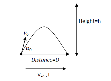
4.8.1 Newtonian Approach

We consider a projectile launched at an angle, with a horizontal distance D between the starting point and the target, and a maximum height h. The gravitational acceleration is g, and the initial velocity of the projectile has components vx0 (horizontal) and vy0 (vertical).

vector_4_8_1en

a) Time and velocity components

The time required for the projectile to travel the distance D with the constant horizontal velocity vx0 is:

\begin{align} v_{x0} = \frac{D}{T} \quad \Rightarrow \quad T = \frac{D}{v_{x0}} \label{eq:R553} \end{align}

To cover the distance D, the projectile also needs an upward velocity, otherwise it will hit the ground too early. This requires an initial velocity component in the y-direction vy0. This velocity is determined by the horizontal distance D and the time T. Thus, T is also the time it takes to go from the ground up and return to the ground.

Because the motion is symmetric, the time to reach the highest point is:

\begin{align} T_{\text{up}} = \frac{T}{2} \label{eq:R554} \end{align}

At this point, the vertical velocity is zero. From the equation of motion:

\begin{align} v_y = v_{y0} - g t = 0 \quad \text{at} \quad t = \frac{T}{2} \label{eq:R555} \end{align}

This yields:

\begin{align} v_{y0} = g t = g \frac{T}{2} = g \frac{D}{2 v_{x0}} \label{eq:R556} \end{align}

b) Height and relation with time

The maximum height is reached at time T/2, thus:

\begin{align} h = v_{y0} \frac{T}{2} - \frac{1}{2} g \left( \frac{T}{2} \right)^2 \label{eq:R557} \end{align}
\begin{align} h = \frac{g D}{2 v_{x0}} \cdot \frac{D}{2 v_{x0}} - \frac{1}{2} g \left( \frac{D}{2 v_{x0}} \right)^2 = \frac{g D^2}{8 v_{x0}^2} \label{eq:R558} \end{align}

Conversely, this gives:

\begin{align} v_{x0} = D \sqrt{\frac{g}{8h}} \label{eq:R559} \end{align}

When the projectile falls from the highest point h, it takes T/2 to reach the ground.

c) Total velocity and trajectory parameters

To reach the highest point:

\begin{align} v_{y0} = g \frac{T}{2} = g \sqrt{\frac{2h}{g}} = \sqrt{2 h g} \label{eq:R560} \end{align}

The total initial velocity is:

\begin{align} v_0^2 = v_{x0}^2 + v_{y0}^2 = \frac{g D^2}{8 h} + 2 h g = g \frac{D^2 + 16 h^2}{8 h} \label{eq:R561} \end{align}
\begin{align} \Rightarrow v_0 = \sqrt{ g \frac{D^2 + 16 h^2}{8 h} } \label{eq:R562} \end{align}

Furthermore:

\begin{align} v_{x0} = v_0 \cos \alpha_0 \label{eq:R563} \end{align}

The launch angle α0 follows from:

\begin{align} \tan \alpha_0 = \frac{v_{y0}}{v_{x0}} = \frac{\sqrt{2 h g}}{D \sqrt{g/(8h)}} = \frac{4 h}{D} \label{eq:R564} \end{align}
\begin{align} \tan \alpha_0 = \frac{4 h}{D} \label{eq:R565} \end{align}

d) Trajectory equation

The y-position as a function of time:

\begin{align} y(t) = v_{y0} t - \frac{1}{2} g t^2 = g \frac{T}{2} t - \frac{1}{2} g t^2 = \frac{1}{2} g t (T - t) \label{eq:R566} \end{align}
\begin{align} y(t) = \frac{1}{2} g t \left( \frac{D}{v_{x0}} - t \right) \label{eq:R567} \end{align}

In terms of the x-position:

\begin{align} x = v_{x0} t \quad \Rightarrow \quad t = \frac{x}{v_{x0}} \label{eq:R568} \end{align}
\begin{align} y(x) = \frac{1}{2} g \frac{x}{v_{x0}} \left( \frac{D}{v_{x0}} - \frac{x}{v_{x0}} \right) = \frac{1}{2} \frac{g}{v_{x0}^2} x (D - x) \label{eq:R569} \end{align}

Thus, the trajectory of the projectile is a parabola:

\begin{align} y(x) = \frac{1}{2} \frac{g}{v_{x0}^2} x (D - x) \label{eq:R570} \end{align}

This is therefore a function of the required distance D when the initial horizontal velocity component \(v_{x0}\) is given.

e) Example calculation

D (m) vx0 (m/s) T (s) h (m) v0 (m/s)
10524.9311.06
105000.020.000493500
10052049399
1005024.9351

(which are calculated using g = 9.87 m/s²)

f) Next step

Now that we have fully developed the Newtonian approach, we can compare it with the calculation based on Schwarzschild geometry within general relativity. This comparison follows in the next section.

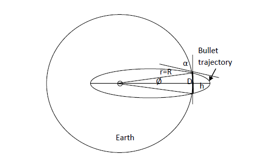
4.8.2 Schwarzschild Approach

For this approach, we consider the projectile trajectory as part of an ellipse, with the center of the Earth coinciding with one of the foci. We use the results from the Schwarzschild equation from chapter 4.7, Alternative Derivation of the Orbit Equation.

For the orbital trajectory, the semi-major axis is given by:

\begin{align} a = \frac{L^2}{G M} \frac{1}{1 - e^2} \label{eq:R571} \end{align}

The parameter e is the eccentricity of the projectile trajectory. The perihelion is:

\begin{align} r_1 = a (1 - e) \label{eq:R572} \end{align}

and the aphelion:

\begin{align} r_2 = a (1 + e) \label{eq:R573} \end{align}
\begin{align}\Rightarrow e = \frac{r_2 - r_1}{r_2 + r_1} \label{eq:R575} \end{align}

For a circle, we therefore have \(e = 0\,\, \text{and} \,\,r = r_1 = r_2 = a\).

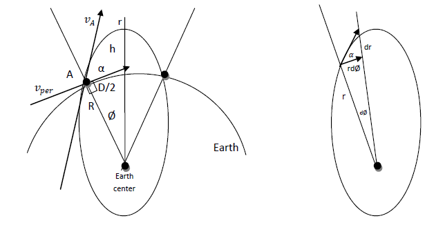
For an ellipse with the Earth's center in the left focus:

\begin{align} r(\phi) = \frac{a (1 - e^2)}{1 - e \cos\!\left[\phi(1-\epsilon)\right]} \label{eq:R576} \end{align}

Angle between velocity and radius vector

We now determine the angle \(α\) between the velocity \(v\) (tangential to the ellipse) and the perpendicular component \(v_{per}\) in order to determine the angular momentum. In this experiment, \(v\) is the total velocity of the projectile along the ellipse, while \(v_{per}\) is the component of the velocity \(v\) relative to the Earth's surface and, as stated, perpendicular to \(r(\phi)\).

\begin{align} \tan \alpha = \frac{1}{r} \frac{dr}{d\phi} \label{eq:R577} \end{align}
\begin{align} \tan \alpha =\frac{\{1-e\cos\left[\phi(1-\epsilon)\right]\}}{a(1-\epsilon^2)}\, \frac{\{a(1-e^2)(1-\epsilon)(e\sin{\left[\phi(1-\epsilon)\right])}\}} {\{1-e\cos\left[\phi(1-\epsilon)\right]\}^2} \label{eq:R578} \end{align}
\begin{align} \tan \alpha =\frac{dr}{rd\phi} =\frac{e(1-\epsilon)\sin{\left[\phi(1-\epsilon)\right]}}{1 - e \cos\left[\phi(1-\epsilon)\right]} \label{eq:R579} \end{align}
\begin{align} \alpha = \arctan\left(\frac{e(1-\epsilon)\sin{\left[\phi(1-\epsilon)\right]}} {1 - e \cos\left[\phi(1-\epsilon)\right]} \right) \label{eq:R580} \end{align}

With:

\begin{align} \cos \alpha = \frac{1}{\sqrt{1 + \tan \alpha}} \label{eq:R581} \end{align}

Then we obtain:

\begin{align} cos{\alpha}=\left[1+ \left( \frac{e(1-\epsilon)\sin{\left[\phi(1-\epsilon)\right]}} {1 - e \cos\left[\phi(1-\epsilon)\right]} \right)^2\right]^{-1/2} \label{eq:R582} \end{align}
\begin{align} cos{\alpha}=\left[ \frac{ 1 - 2 e \cos\left[\phi(1-\epsilon)\right] + e^2 \cos^2\left[\phi(1-\epsilon)\right] + \{e(1-\epsilon)\sin\left[\phi(1-\epsilon)\right] \}^2 }{\{1 - e \cos\left[\phi(1-\epsilon)\right]\}^2} \right]^{-1/2} \label{eq:R583} \end{align}

Because of the negative exponent, we invert the expression:

\begin{align} cos{\alpha}= \frac{1 - e \cos\left[\phi(1-\epsilon)\right]}{\left[ 1 - 2 e \cos\left[\phi(1-\epsilon)\right] + e^2 \cos^2\left[\phi(1-\epsilon)\right] + (1-2\epsilon+\epsilon^2)e^2\sin^2\left[\phi(1-\epsilon)\right]\right]^{1/2}} \label{eq:R584} \end{align}
\begin{align} cos{\alpha}= \frac{1 - e \cos\left[\phi(1-\epsilon)\right]}{\left[ 1 - 2 e \cos\left[\phi(1-\epsilon)\right] + e^2 \cos^2\left[\phi(1-\epsilon)\right] +e^2\sin^2\left[\phi(1-\epsilon)\right]-\epsilon (2-\epsilon)e^2\sin^2\left[\phi(1-\epsilon)\right]\right]^{1/2}} \label{eq:R585} \end{align}
\begin{align} cos{\alpha}= \frac{1 - e \cos\left[\phi(1-\epsilon)\right]} {\left[ 1 - 2 e \cos\left[\phi(1-\epsilon)\right] +e^2(1-\epsilon (2-\epsilon)\sin^2\left[\phi(1-\epsilon)\right])\right]^{1/2}} \label{eq:R586} \end{align}

Angular momentum

The angular momentum L is constant along the ellipse and is given by:

\begin{align} L = v_{per}\cdot r = v \cdot \cos \alpha \cdot \, r \label{eq:R587} \end{align}

At the starting point on the Earth's surface:

\begin{align} L = v_{x0}\cdot R_{\text{earth}} \label{eq:R588} \end{align}

According to the Schwarzschild solution:

\begin{align} L = \sqrt{a G M (1 - e^2)} \label{eq:R589} \end{align}

Velocity along the ellipse

\begin{align} v = \frac{L}{r \cos \alpha} = \frac{\sqrt{aG M(1 - e^2)}}{a(1-e^2)\,\cos{\alpha}} (1-e\cos\left[\phi(1-\epsilon)\right]) \label{eq:R590} \end{align}

This simplifies to:

\begin{align} v = \sqrt{\frac{G M}{a (1 - e^2)}}\, \frac{1 - e \cos\!\left[\phi(1-\epsilon)\right])} {\cos \alpha} \label{eq:R591} \end{align}

Substitute \(\cos{\alpha}\) from equation (\ref{eq:R586}) into equation (\ref{eq:R591}):

\begin{align} v = \left(\frac{G M}{a (1 - e^2)}\right)^{1/2}\,\frac{1-e\cos\left[\phi(1-\epsilon)\right]}{1-e\cos\left[\phi(1-\epsilon)\right]} (1 - 2 e \cos\!\left[\phi(1-\epsilon)\right] + e^2\{1-\epsilon(2-\epsilon) \sin^2\!\left[\phi(1-\epsilon)\right]\})^{1/2} \label{eq:R592} \end{align}

The instantaneous velocity as a function of \(\phi\) is:

\begin{align} v = \sqrt{\left(\frac{G M}{a (1 - e^2)}\right)\, (1 - 2 e \cos\!\left[\phi(1-\epsilon)\right] + e^2\{1-\epsilon(2-\epsilon) \sin^2\!\left[\phi(1-\epsilon)\right]\})} \label{eq:R593} \end{align}

Relativistic correction parameter

Obtained from the previous chapter \(\epsilon\):

\begin{align} \epsilon = \frac{3 (G M)^2}{c^2 L^2} = \frac{3 (G M)^2}{c^2 aGM(1-e^2)} = \frac{3 G M}{c^2 a (1 - e^2)} \label{eq:R594} \end{align}

Here:

\begin{align} \epsilon = \frac{3 (G M)^2}{c^2 L^2} = \frac{3 (G M)^2}{c^2 (v_{x0}R_{earth})^2} = \frac{3c^2}{v_{x0}^2} \left( \frac{G M}{c^2 R_{earth}} \right)^2 \,\,\text{this is dimensionless} \label{eq:R595} \end{align}

Geometric relations

vector_4_8_2a

To zoom in further:

vector_4_8_2b

\begin{align} \phi \cdot R=\frac{D}{2} \Rightarrow \phi=\frac{D}{2R} \label{eq:R596} \end{align}
\begin{align} v_{per} = v_{xA} = v\cos(\alpha) \,\,\text{and}\,\, v_{yA} = v\sin(\alpha) \label{eq:R597} \end{align}

From (\ref{eq:R576}):

\begin{align} a(1 - e^{2}) = r\{1 - e\cos\left[\phi\,(1 - \epsilon)\right]\} \label{eq:R598} \end{align}

From (\ref{eq:R593}):

\begin{align} v = \sqrt{\left(\frac{G M}{a (1 - e^2)}\right)\, (1 - 2 e \cos\!\left[\phi(1-\epsilon)\right] + e^2\{1-\epsilon(2-\epsilon) \sin^2\!\left[\phi(1-\epsilon)\right]\})} \label{eq:R599} \end{align}
\begin{align} v^2 = \left(\frac{G M}{a (1 - e^2)}\right)\, (1 - 2 e \cos\!\left[\phi(1-\epsilon)\right] + e^2\{1-\epsilon(2-\epsilon) \sin^2\!\left[\phi(1-\epsilon)\right]\}) \label{eq:R600} \end{align}
\begin{align} v^2 =GM \,\frac{ (1 - 2 e \cos\!\left[\phi(1-\epsilon)\right] + e^2\{1-\epsilon(2-\epsilon) \sin^2\!\left[\phi(1-\epsilon)\right]\}) }{r\{1 - e \cos\!\left[\phi(1-\epsilon)\right]\}} \label{eq:R601} \end{align}
\begin{align} \frac{v^2r}{GM}\,\{1 - e \cos\left[\phi(1-\epsilon)\right]\}= 1 - 2 e \cos\!\left[\phi(1-\epsilon)\right] + e^2\{1-\epsilon(2-\epsilon) \sin^2\!\left[\phi(1-\epsilon)\right]\} \label{eq:R602} \end{align}
\begin{align} e^2\{1-\epsilon(2-\epsilon) \sin^2\!\left[\phi(1-\epsilon)\right]\}- e \cos\left[\phi(1-\epsilon)\right]\left(2-\frac{v^2r}{GM}\right) +\left(1-\frac{v^2r}{GM}\right)=0 \label{eq:R603} \end{align}
\begin{align} e=\frac{\cos\left[\phi(1-\epsilon)\right]\left(2-\frac{v^2r}{GM}\right)} {2\{1-\epsilon(2-\epsilon) \sin^2\!\left[\phi(1-\epsilon)\right]\}}\pm \label{eq:R605} \end{align}
\begin{align} \pm\frac{ \sqrt{ \left[\cos \left[\phi(1-\epsilon)\right]\left(2-\frac{v^2r}{GM}\right)\right]^2-4\left(1-\frac{v^2r}{GM}\right) \{1-\epsilon(2-\epsilon) \sin^2\!\left[\phi(1-\epsilon)\right]\}\ }} {2\{1-\epsilon(2-\epsilon) \sin^2\!\left[\phi(1-\epsilon)\right]\}} \label{eq:R606} \end{align}

For the starting point at the intersection of the Earth and the trajectory, we have \(r=R\). (\(R\) here is the radius of the Earth) and \(\phi=\frac{D}{2R}\).

From (576):

\begin{align} r=\frac{a(1-\epsilon^2)}{1-e\cos\left[\phi(1-\epsilon)\right]} \label{eq:R607} \end{align}
\begin{align} a(1-\epsilon^2)=R\left\{1-e\cos\left[\frac{D}{2R}(1-\epsilon)\right]\right\} \label{eq:R608} \end{align}
\begin{align} a=\frac{R\left\{1-e\cos\left[\frac{D}{2R}(1-\epsilon)\right]\right\}}{(1-\epsilon^2)} \label{eq:R609} \end{align}
\begin{align} e=\frac{\cos\left[\phi(1-\epsilon)\right]\left(2-\frac{v^2r}{GM}\right)} {2\{1-\epsilon(2-\epsilon) \sin^2\!\left[\phi(1-\epsilon)\right]\}}\pm \label{eq:R611} \end{align}
\begin{align} \pm\frac{ \sqrt{ \left[\cos \left[\phi(1-\epsilon)\right]\left(2-\frac{v^2r}{GM}\right)\right]^2-4\left(1-\frac{v^2r}{GM}\right) \{1-\epsilon(2-\epsilon) \sin^2\!\left[\phi(1-\epsilon)\right]\}\ }} {2\{1-\epsilon(2-\epsilon) \sin^2\!\left[\phi(1-\epsilon)\right]\}} \label{eq:R612} \end{align}

Or from equations (\ref{eq:R571}), (\ref{eq:R595}) and (\ref{eq:R609}):

\begin{align} R\left\{1 - e\cos\left[\frac{D}{2R}(1 - \epsilon)\right]\right\} = a(1 - e^{2}) = \frac{L^{2}}{GM} \label{eq:R613} \end{align}

\begin{align} e=\frac{1-\frac{L^{2}}{RGM}}{\cos\left[\frac{D}{2R}(1 - \epsilon)\right]}= \frac{1-\frac{L^{2}}{RGM}}{\cos\left[\frac{D}{2R}\left(1 - \frac{3c^2}{v_{x0}^2}\left(\frac{GM} {c^2R_{earth}}\right)^2\right)\right]} = \frac{1-\frac{(v_{x0}R)^{2}}{RGM}}{\cos\left[\frac{D}{2R}\left(1 - \frac{3c^2}{v_{x0}^2}\left(\frac{GM} {c^2R_{earth}}\right)^2\right)\right]} \label{eq:R614} \end{align}
\begin{align} e= \frac{1-\frac{(v_{x0}R)^{2}}{RGM}}{\cos\left[\frac{D}{2R}\left(1 - \frac{3c^2}{v_{x0}^2}\left(\frac{GM} {c^2R_{earth}}\right)^2\right)\right]} \label{eq:R615} \end{align}

The given velocity at the point \( r = R \) is \( v \). Thus, for a given velocity, there are two solutions for \( e \).

Here, \( h \) is the highest point of the projectile trajectory:

\begin{align} h = a(1 + e) - R \label{eq:R616} \end{align}

Together with (3):

\begin{align} h = \frac{R\left\{1 - e\cos\left[\frac{D}{2R}\left(1 - \epsilon\right)\right]\right\}} {1 - e^{2}}(1 + e) - R= R\left\{\frac{1 - e\cos\left[\frac{D}{2R}\left(1 - \epsilon\right)\right]} {1 - e} - 1\right\} \label{eq:R617} \end{align}
\begin{align} h = R\left\{\frac{1 - e\cos\left[\frac{D}{2R}\left(1 - \epsilon\right)\right]-1+\epsilon} {1 - e}\right\} = R\frac{e\left(1 - e\cos\left[\frac{D}{2R}\left(1 - \epsilon\right)\right]\right)} {1 - e} \label{eq:R618} \end{align}

Here, \( D \) is the horizontal distance of the projectile on Earth, \( v \) is the initial velocity of the projectile, and \( R \) is the Earth's radius. As seen above:

\begin{align} \phi = \frac{D}{2R}. \label{eq:R619} \end{align}

Or pragmatically, in our projectile example with \( v_{x0} \) and \( D \) as starting parameters:

\begin{align} h = a(1 + e) - R = a\frac{1 - e^{2}}{1 - e} - R = \frac{L^{2}}{GM}\frac{1}{1 - e} - R \label{eq:R620} \end{align}

\begin{align} = \frac{v_{x0}^{2} R^{2}}{GM}\frac{1}{1 - e} - R \label{eq:R621} \end{align}

Where:

\begin{align} e = \frac{1 - \frac{v_{x0}^{2} R}{GM}}{\cos\left[\frac{D}{2R} \left(1 - \frac{3c^{2}}{v_{x0}^{2}}\left(\frac{GM}{ c^{2} R}\right)^2\right)\right]} \label{eq:R622} \end{align}

Derivation of the circumference of an ellipse

\begin{align} \frac{x^{2}}{a^{2}} + \frac{y^{2}}{b^{2}} = 1, \qquad x = a\cos\beta,\quad y = b\sin\beta \label{eq:R623} \end{align}

\begin{align} \text{Circumference} = 4a \int_{0}^{\pi/2} \sqrt{ \left(\frac{dx}{d\beta}\right)^{2} + \left(\frac{dy}{d\beta}\right)^{2} } \, d\beta \label{eq:R624} \end{align}

\begin{align} = 4a \int_{0}^{\pi/2} \sqrt{ a^{2}\sin^{2}\beta + b^{2}\cos^{2}\beta } \, d\beta \label{eq:R625} \end{align}

\begin{align} = 4a \int_{0}^{\pi/2} \sqrt{ a^{2}(1-\cos^2\beta) + b^{2}\cos^{2}\beta } \, d\beta \label{eq:R626} \end{align}

\begin{align} = 4a \int_{0}^{\pi/2} \sqrt{ a^{2} - (a^{2} - b^{2})\cos^{2}\beta } \, d\beta \label{eq:R627} \end{align}

\begin{align} \text{Circumference} = 4a \int_{0}^{\pi/2} \sqrt{ 1 - e^{2}\cos^{2}\beta } \, d\beta \label{eq:R628} \end{align}

There is no simple closed-form solution for the circumference of an ellipse. A well-known approximation is Ramanujan’s formula:

\begin{align} \text{Circumference} \approx \pi a \left[ 3(1 + \sqrt{1 - e^{2}}) - \sqrt{10\sqrt{1 - e^{2}} + 3(2 - e^{2})} \right] \label{eq:R629} \end{align}

Summary of formulas used

The starting points for this derivation are the velocity of the projectile along the Earth's surface (\(v_{x0}=v_{per}\), perpendicular to \(r\)) and the required distance \(D\). Thus, at the starting point where the projectile is launched, we know the position and momentum of the projectile and should be able to calculate the trajectory.

  • \( L = v_{x0}\cdot R_{\text{Earth}} \hspace{13em}\text{thus}\,\,\epsilon\, \text{is a function of }L\left(v_{x0}\right) \)
  • \( \epsilon = \dfrac{3 (G )^2M}{2 c^2 L^2} \hspace{14em}\text{thus}\,\,\epsilon\left(v_{x0}\right) \)
  • \( \phi = \dfrac{D}{2R} \hspace{16em}\text{thus}\,\,\phi\left(D\right)\)
  • \( e = \dfrac{1 - \frac{L^{2}}{RGM}} {\cos\!\left[\phi(1 - \epsilon)\right]} \hspace{12em}\text{thus}\, \,e\left(v_{x0},D\right)\)
  • \( \alpha = \arctan\!\left\{ \dfrac{e\,(1 - \epsilon)\sin\left[\phi(1 - \epsilon)\right]} {1 - e\,\cos\left[\phi(1 - \epsilon)\right]} \right\} \hspace{4em}\text{thus}\,\,e\left(v_{x0},D\right) \)
  • \( a = \dfrac{L^2}{G M (1-e^2)} \hspace{12em}\text{thus}\,\,a\left(v_{x0},D\right) \)
  • \( h = a(1+e) - R \hspace{12em} \text{thus}\,\,h\left(v_{x0},D\right) \)

With these formulas, starting from the initial velocity and required distance, the full trajectory and maximum height of the projectile can be calculated relativistically.

Detailed results of calculations

Detailed results of calculations for the example above. The starting parameters are the (perpendicular to r) velocity of the projectile and the required distance.

Newton Schwarzschild
Parameter 5 m/s 500 m/s 500 m/s 1000 m/s 5 m/s 500 m/s 500 m/s 1000 m/s
Distance (m) 101020002000 101020002000
vr0 (m/s) 9.870.1019.739.87 9.760.1019.669.71
Velocity (m/s) 115005001000 115005001000
\(\epsilon\) ---- 5.25×10⁻³ 5×10⁻⁷ 5.25×10⁻⁷ 1×10⁻⁷
e (eccentricity) 1.0000.9960.9960.984
a (m) 3.18×10⁶ 3.18×10⁶ 3.18×10⁶ 3.20×10⁶
h (m) 4.934.93×10-4 19.734.93 4.884.91×10-4 19.664.85
α (rad) 1.100.0000.040.010 1.100.0000.040.010
α (deg) 63.130.01132.260.565 62.880.01132.250.556
Φ (rad) 7.87×10⁻⁷ 7.87×10⁻⁷ 1.57×10⁻⁴ 1.57×10⁻⁴
L (angular momentum) 3.18×10⁷ 3.18×10⁹ 3.18×10⁹ 6.36×10⁹ 3.18×10⁷ 3.18×10⁹ 3.18×10⁹ 6.36×10⁹
cos(α) 0.45201.00000.99921.0000 0.45581.00000.99921.0000
cos(α + Φ) 0.45581.0000.99921.000
Circumference (km) ---- 12662128941289413346

3) Analysis of the results

Height differences

In the classical case, the maximum height of the projectile is \( h \approx 4.93 \,\text{m} \) at low velocities. In the Schwarzschild approach, this is slightly lower (for example \( h \approx 4.88 \,\text{m} \)), indicating a stronger effective gravitational field.

Eccentricity

An eccentricity of exactly \( e = 1 \) implies the classical parabola. The Schwarzschild approach shows that the trajectories are slightly elliptical with \( e < 1. \) For a horizontal velocity of 500 m/s, we find \( e \approx 0.996, \) while at 5 m/s \( e \approx 1, \) which corresponds to an almost parabolic trajectory.

Direction angle

The deviation in direction angle \( \Phi \) is very small at low velocities, but becomes measurable at higher energies. For a projectile of 500 m/s over 2 km, the deviation is \( \Phi \approx 1.57 \times 10^{-4} \,\text{rad}, \) which corresponds to a precession of the ellipse axis.

Angular momentum and circumference

The angular momentum \( L \) increases with the initial velocity. The corresponding (approximate) circumference of the elliptical orbit also increases, reflecting the longer path traveled by a high-energy projectile.

4.8.3 Conclusion

  • Newtonian ballistics is an excellent approximation for everyday situations.
  • Relativistic corrections are subtle but indispensable for highly precise applications and at high velocities.
  • The Schwarzschild approach shows that even a simple projectile trajectory is, in principle, influenced by the curvature of spacetime.