Part II – Derivation of General Relativity
2 General Relativity
Before Einstein formulated his famous general theory of relativity in 1915, he first developed the special theory of relativity in 1905 (see Appendix 9). In this theory, he considered only coordinate systems moving uniformly, that is, with constant velocity relative to one another. The influence of masses — and thus gravity — was not yet taken into account.
The special theory of relativity is based on two fundamental principles:
- The speed of light in vacuum is the same in every coordinate system and equals: \( c = 299\,792\,458 \,\text{m/s} \).
- The laws of physics are valid in every inertial (non-accelerating) reference frame.
In Newton’s classical theory, time was assumed to be universal: time intervals are identical in both stationary and moving systems. However, special relativity showed that this is not correct. In a moving system, time intervals proceed more slowly than in a stationary system, an effect known as time dilation.
The length of an object also changes due to motion: it decreases relative to its original rest length. This effect is called length contraction. Both phenomena are discussed in detail in Appendix 9.
These results are direct consequences of the fact that the speed of light is constant for all observers, regardless of their motion. Since time and space depend on the chosen frame of reference, Einstein unified these quantities into a single entity: spacetime.
One of the most well-known results of this theory is the famous mass–energy relation:
in which energy and mass are considered equivalent (see Appendix 9.9). In a later stage, Einstein focused on extending his theory to accelerated frames and the influence of mass. This led in 1915 to the formulation of general relativity, in which gravity is no longer treated as a force, but as a consequence of the curvature of spacetime.
For a first impression of Einstein’s final field equations, we refer to chapter 2.16, where a summary of the final formula is given. The following chapters will discuss step by step the concepts and mathematical derivations that lead to these results.
2.1 The Equivalence Principle
By studying the influence of masses, Newton formulated the law of gravitation: masses experience acceleration due to an attractive force. When comparing gravity with other fundamental forces, such as the electric and magnetic force, both similarities and important differences become apparent.
2.1.1 Electric force
The electric force arises from charges on two particles \( q_{1} \) and \( q_{2} \). Depending on the sign of the charges, they attract or repel each other. The force between the particles is given by Coulomb’s law:
where \( k_{e} \) is the electric constant and \( r \) is the distance between the charges. The resulting acceleration depends on the mass of the particle:
There is therefore an attractive force due to the charges, but the acceleration is determined by both the magnitude of the masses and the interaction.
2.1.2 Magnetic force
Magnetic forces also cause acceleration. This depends on the charge of the particle, the orientation and strength of the magnetic field, and the mass of the particle.
2.1.3 Gravity
The gravitational force between two masses \( m_{1} \) and \( m_{2} \) is given by Newton as:
where \( G \) is the gravitational constant. By analogy with the electric force, one might expect a distinction between gravitational mass \( m_{\text{grav}} \), which produces the force, and inertial mass \( m_{\text{inert}} \), which undergoes acceleration.
At first glance, there is no reason why \( m_{\text{inert},1} \equiv m_{\text{grav},1} \) should hold. However, experiments by Eötvös (around 1885) show that these two masses are always equal.
Another important difference with the electric force is that gravity has no positive or negative charge: the force between two masses is always attractive.
Due to the equality of gravitational and inertial mass, it follows that:
The mass \( m \) of the falling object cancels out, so that the acceleration depends only on \( M \), the mass of the attracting body (for example, the Earth). This means that all objects, regardless of their mass, fall with the same acceleration, provided that air resistance is neglected.
This leads to the conclusion that the motion of an object in a gravitational field is not determined by its own mass, but by the geometry of spacetime in which it moves.
2.1.4 Einstein’s Thought Experiment
Inspired by this observation, Einstein imagined two situations:
- A person standing still on Earth experiences a gravitational acceleration \( g = 9{,}81 \,\text{m/s}^{2} \).
- A person is inside an accelerating rocket (with the same acceleration \( g \)) in empty space.
According to Einstein, these situations are locally indistinguishable, the person experiences the same effect in both cases. This led to the equivalence principle: gravity and inertia are locally equivalent. Einstein concluded that gravity is not a force, but a manifestation of the curvature of spacetime caused by mass.
2.1.5 Remark
The mass \( m \) also exerts a force on \( M \), with the following acceleration:
However, since usually \( M \gg m \), the acceleration of \( M \) is negligible. The forces are equal and opposite (Newton’s third law).
In classical theory, only masses exert forces on each other. This would imply that a mass has no influence on massless particles such as photons. General relativity, however, states that masses curve spacetime, and that all objects, even massless ones, follow this curvature. Therefore, light is also deflected in a gravitational field.
2.1.6 Confirmation by Observation
In 1919, Arthur Eddington confirmed this effect experimentally: during a solar eclipse, he observed that stars near the edge of the Sun appeared shifted, exactly as Einstein had predicted. The derivation of this effect will follow in a later experimental chapter.
2.1.7 Key Insights
- Gravity versus other forces: While forces such as the electric force depend on both mass and charge, gravity is unique because all objects, regardless of their mass, experience the same acceleration in a gravitational field.
- Gravitational and inertial mass are equal: Experiments show that the mass that produces gravity (gravitational mass) is equal to the mass that responds to a force (inertial mass).
- Acceleration independent of mass: As a result, all objects fall with the same acceleration, which is not generally the case for other forces.
- Einstein’s thought experiment: A person in an elevator on Earth experiences the same as someone in an accelerating rocket in empty space → local equivalence between gravity and acceleration.
- Consequence: Gravity is no longer viewed as a force, but as a result of the curvature of spacetime.
2.1.8 Intuitive Explanation
Imagine you are inside a closed space, a rocket or a room without windows. If you feel yourself being pressed against the floor, you cannot determine whether you are on Earth (where gravity pulls you downward) or in space inside a rocket that is accelerating. This is the essence of the equivalence principle.
Einstein argued that if you cannot detect the difference, then physically there is no difference at that moment and location. What we call gravity is therefore essentially an effect of acceleration, or conversely, acceleration cannot locally be distinguished from gravity. Instead of viewing gravity as a force (as Newton did), general relativity describes gravity as a deformation of spacetime. Mass “warps” spacetime, and objects follow this curvature.
2.2 Curvature of Spacetime
To understand the significance of the transition from Newton’s classical gravitational model to Einstein’s geometric model, we first approach the subject in an alternative, more intuitive way.
Consider a particle in free space, far away from masses and without the influence of external forces. In such a situation, the particle continues to move with constant velocity in a straight line, a principle already described around 1600 by Galileo Galilei.
If we imagine spacetime as consisting of rectangular grid lines, a spatial reference framework without curvature, the particle follows a straight path along this grid. There is nothing to cause deviation from its initial direction or velocity.
Einstein proposed that this picture changes in the presence of a large mass. That mass deforms the structure of spacetime, causing the “straight” lines of the grid to become curved. Instead of gravity acting as a force, the particle naturally moves along these curved lines.
The closer the particle comes to the mass, the more its path deviates from its original straight line. Yet the particle does not feel a force: it moves freely, but follows the curvature of space. This path turns out to be a kind of “straight line” within the curvature, and is referred to later in this document as a geodesic.
In general relativity, therefore, there is no gravitational force as in Newton’s theory; instead, the effect of gravity arises from the geometry of spacetime itself.
2.2.1 From Force to Geometry
The challenge Einstein faced was to find a mathematical description of this curvature. He sought a way to express the geometry of spacetime as a function of mass and energy, in a manner independent of the chosen coordinate system.
This meant developing a fully coordinate-independent formulation, so that the laws of physics retain the same form in every frame, a central principle of general relativity. The effects of mass and energy on geometry would ultimately be encoded in the Einstein field equations, which describe how matter curves spacetime and how curved spacetime determines the motion of matter.
2.2.2 Independence of the Chosen Coordinate System
To determine the position of a point in space, we always need a reference, an origin from which distances are measured. A common method is to choose a Cartesian coordinate system with three mutually perpendicular axes: the x-, y-, and z-axes.
We can describe the location of a point using coordinates \( (x, y, z) \), where these values represent distances from the origin along the respective axes. The distance from that point to the origin is then, according to the Pythagorean theorem:
If we choose a different coordinate system (with a different origin or rotation), the coordinate values, and thus \( s \), change. However, if we consider not the absolute position of a single point, but the infinitesimal distance between two nearby points, that distance remains invariant under coordinate transformations. This differential distance is denoted by:
This formula is applicable in an orthogonal, flat, Cartesian coordinate system. To generalize it, including situations in which the axes are not necessarily perpendicular, a more fundamental approach based on vector analysis is required.
2.2.3 Vector Approach to Distance
We can interpret the differential displacement as the sum of three vector components:
Here, \(\hat{e}_x\) denotes the unit vector along the x-axis, and \(dx\) represents its magnitude.
In Figure 2.3, it is schematically illustrated how the vector \( d\vec{s} \) can be decomposed into components along the basis vectors of the chosen coordinate system.
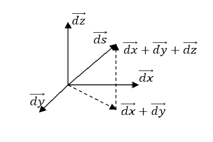
The magnitude \( ds \) of the vector \( d\vec{s} \) is obtained via the inner product \(d\vec{s} \cdot d\vec{s}\):
Reminder: the inner product of two vectors \( \vec{A} \) and \( \vec{B} \) is:
where \( \varphi \) is the angle between the two vectors.
And thus:
For the full inner product of \( d\vec{s} \), we obtain:
Or more compactly:
In an orthogonal system, the cross terms such as \( d\vec{x} \cdot d\vec{y} \) vanish, since the angles between the axes are 90° and \( \cos 90^\circ = 0 \). In that case, we simply obtain:
In a non-orthogonal coordinate system, the angles between the axes are not necessarily 90°, so the cross terms also contribute. The general form then becomes:
The coefficients \( g_{ij} \) provide information about the relative orientation of the axes and together form the metric tensor \( g_{ij} \).
2.2.4 Extension to Spacetime
Einstein sought an even more general formulation, for a four-dimensional system consisting of one time axis and three spatial axes. These axes need not be orthogonal, and moreover the metric may vary from point to point in spacetime. The general expression for the square of the spacetime interval is then:
Or in Einstein notation:
where:
- \( \mu, \nu = 0, 1, 2, 3 \)
- \( x^{0} = ct,\; x^{1} = x,\; x^{2} = y,\; x^{3} = z \)
- \( g_{\mu\nu} \) are the components of the four-dimensional metric tensor
In Einstein notation (where summation over repeated indices, so-called “dummy indices”, is implied), the sum is not written explicitly.
2.2.4.1 Expansion of the Sum
When we fully expand the expression (\ref{eq:R19}) for all values of \( \mu \) and \( \nu \), we obtain:
This is the four-dimensional counterpart of the earlier three-dimensional expression (\ref{eq:R2242}) (see chapter 5 for more details).
2.2.4.2 Remark on Symmetry
The metric tensor \( g_{\mu\nu} \) is symmetric, meaning:
Therefore, the tensor contains only 10 independent components instead of 16. This makes it mathematically elegant and practically manageable.
2.2.5 Key Insights
- Free motion in flat space: A particle unaffected by forces moves in a straight line with constant velocity (inertial motion).
- Spacetime as geometry: In Einstein’s view, mass deforms the structure of spacetime, causing “straight lines” (inertial paths) to become curved.
- Gravity = curvature: Instead of a force (as in Newtonian physics), gravity arises from the curvature of spacetime.
- Geodesics: Objects follow the “straightest” possible paths in curved spacetime, even if these appear curved to an external observer.
- Einstein’s challenge: Develop a coordinate-independent mathematical description of how mass curves spacetime → Einstein field equations.
For further details on tensors and the metric, and their application to specific cases such as the Schwarzschild solution, see chapter 5.
2.2.6 Intuitive Explanation
Imagine the following:
- A billiard ball rolls across a smooth, flat table, it moves in a straight line.
- Now place a heavy sphere on a flexible rubber sheet (like a trampoline), creating a curvature.
- If you roll a smaller ball across the sheet, it will be deflected by the deformation, even though no force is directly applied.
According to Newton, gravity is a force acting at a distance. According to Einstein, there is no force: objects move along straight paths, but these paths lie in a curved spacetime. In this sense, a falling apple is not being pulled, but simply follows the shortest path through a curved spacetime.
2.3 Covariant and Contravariant Vectors and Dual Vectors
In general relativity, the concepts of contravariant and covariant frequently appear. In this section, we explain these concepts and show how they arise from the way vectors and fields transform under a change of coordinate system.
As discussed earlier, physical quantities – such as vectors, tensors, and fields – must be independent of the chosen coordinate system. When transforming to another system (for example via rotation or translation), the physical properties remain unchanged, but their components change in a specific way: they transform according to well-defined rules, depending on the type of object (covariant or contravariant).
2.3.1 Scalar Quantities, Vectors, and Fields
A scalar quantity, such as temperature, has a value at each location but no direction. A collection of scalars over space forms a scalar field.
When such a field exhibits a directional variation (for example, a temperature increase in a particular direction), we can take its derivative. This derivative behaves as a vector, and in this specific case we speak of a dual vector.
A dual vector depends on the chosen coordinate system: under a transformation, the components of the vector change in such a way that the overall physical description remains consistent. Because these components transform along with the coordinate system, they are called covariant.
An “ordinary” vector (such as velocity or acceleration) behaves differently: when the coordinate system changes, the underlying vector remains physically the same, but its components transform in the opposite way relative to the basis vectors. Such vectors are called contravariant.
2.3.1.1 Notation and Definitions
To distinguish between the two types of vectors, the following notation is conventionally used:
- A contravariant vector has an upper index: \( A^{\mu} \).
- A covariant vector has a lower index: \( A_{\mu} \).
These are related via the metric tensor \( g_{\mu\nu} \) according to:
The contraction of a contravariant vector with its covariant counterpart yields a scalar invariant:
This expression means that the inner product of a vector with its dual (or “lowered”) version results in a quantity \( I \) that remains invariant under coordinate transformations. This quantity \( I \) can be interpreted as the norm or the squared interval in spacetime, depending on its sign:
- Timelike: \( I > 0 \)
- Spacelike: \( I < 0 \)
- Lightlike: \( I = 0 \)
This classification shows how the metric tensor plays a key role: it not only determines how vector components are transformed, but also how distances, lengths, and causal structures in curved spacetime are defined. Here the signature convention (+,−,−,−) is used, where the time component contributes positively and the spatial components negatively.
2.3.2 Transformations Between Coordinate Systems
Suppose we work in a coordinate system with coordinates \( x^{m} \) (where \( m = 0,1,2,3 \)), and we transform to a new coordinate system with coordinates \( y^{n} \). The relation between the two systems is given by:
In Einstein notation, where summation over repeated indices (from 0 to 3) is implicit, this becomes:
2.3.2.1 Example: Derivative of a Scalar Function
Consider a scalar function \( \varphi \). Its differential is:
Fully expanded:
In the new coordinate system \( y^{n} \), we use the chain rule to transform the components of the derivative:
It follows that the components transform as:
where:
- \( A_{n}(y) = \dfrac{d\varphi}{dy^{n}} \): the covariant vector in the \(y\)-system,
- \( B_{m}(x) = \dfrac{\partial \varphi}{\partial x^{m}} \): the covariant vector in the \(x\)-system.
This is a covariant transformation.
2.3.2.1.1 Fully Expanded (Matrix Form)
In matrix form, equation (\ref{eq:R23215}) becomes:
2.3.2.2 Contravariant Transformation
For contravariant vectors, the transformation formula is reversed:
Fully written out in matrix form:
2.3.3 Transformation Behavior of Basis Vectors
In tensor calculus, it is important not only to understand how the components of a vector change under a coordinate transformation, but also how the associated basis vectors themselves transform.
When changing coordinates from \( x^{m} \) to \( y^{n} \), the corresponding basis vectors are:
- \( \vec e_{m} = \dfrac{\partial}{\partial x^{m}} \)
- \( \vec f_{n} = \dfrac{\partial}{\partial y^{n}} \)
The relationship between basis vectors in different coordinate systems follows from the chain rule of calculus:
It follows that the basis vectors transform covariantly: they change along with the coordinate system. The components of contravariant vectors must therefore adjust in the opposite way to keep the overall object physically invariant.
2.3.3.1 Remark on Einstein Notation
Einstein notation makes use of repeated indices (so-called dummy indices), where summation is automatically implied over the values 0 through 3:
In this section, many expressions are written out explicitly to clarify the meaning of this notation. In later chapters, we will more frequently use the compact Einstein notation.
2.3.4 Key Points
- Scalars versus vectors:
- A scalar quantity (such as temperature) does not change under a coordinate transformation.
- A vector has both direction and magnitude. The components of a vector do change under transformation, depending on the type of vector.
- Contravariant vectors (such as position or velocity vectors \( W^{n} \)):
- Transform opposite to the basis vectors in order to keep the vector physically invariant.
- Transformation formula:
\begin{align} W^{n}(y) = \frac{dy^{n}}{dx^{m}} B^{m}(x) \end{align}
- Covariant vectors (such as dual vectors \( A_{n} \)):
- Transform along with the coordinate system.
- Transformation formula:
\begin{align} A_{n}(y) = \frac{dx^{m}}{dy^{n}} B_{m}(x) \end{align}
- Duality:
- Covariant vectors can be interpreted mathematically as linear functionals on vectors; they belong to the dual vector space.
- Conversion between covariant and contravariant:
- Using the metric tensor \( g_{\mu\nu} \), we can convert between contravariant and covariant vectors:
\begin{align} A_{\mu} = g_{\mu\nu} A^{\nu}, \quad A^{\mu} = g^{\mu\nu} A_{\nu} \end{align}
- Using the metric tensor \( g_{\mu\nu} \), we can convert between contravariant and covariant vectors:
2.3.5 Intuitive Explanation
Imagine standing on a hill and measuring the slope in different directions. The hill itself does not change when you rotate your coordinate axes, but the numerical values describing the slope do. This is precisely the essence of tensor transformations: the direction of a vector remains physically the same, but the coordinates used to describe it change with the reference frame.
The metric acts as a kind of converter between the two types of vectors. You can think of the metric as a ruler that measures differently in each direction, depending on the local curvature of spacetime.
Comparison Table
| Property | Contravariant | Covariant |
|---|---|---|
| Index position | Upper \( A^{\mu} \) | Lower \( A_{\mu} \) |
| Transforms… | Opposite to basis | Along with basis |
| Example | Position, velocity | Gradient, differential |
| Origin | Direction in space | Directional derivative of a scalar field |
2.4 Covariant and Contravariant Transformations of Tensors
In general relativity, and more broadly in tensor analysis, covariant, contravariant, and mixed tensors play a central role. The way these tensors transform under a change of coordinate system is essential for formulating physical laws in a coordinate-independent manner. In this section, we discuss the transformation properties of the different types of tensors.
The transformation rules discussed here form a direct extension of the rules for vectors from the previous section.
2.4.1 Covariant Tensors
A covariant tensor has one or more lower indices, such as \( T_{mn} \), and can be constructed from the product of covariant vectors \( A_{m} \) and \( B_{n} \).
The transformation of a covariant tensor from a coordinate system \(x\) to a new system \(y\) proceeds as follows:
The result of the transformation from \( T_{rs} \) to \( T_{mn} \) is then given by:
Here:
- \( T_{mn}(y) \): the covariant tensor in the new coordinate system \(y\),
- \( \dfrac{dx^{r}}{dy^{m}} \) and \( \dfrac{dx^{s}}{dy^{n}} \): the Jacobian components of the transformation from \(y\) to \(x\),
- \( T_{rs}(x) \): the original covariant tensor in the old system.
2.4.2 Contravariant Tensors
A contravariant tensor has one or more upper indices, such as \( T^{mn} \), and can be constructed from contravariant vectors \( A^{m} \) and \( B^{n} \).
The transformation is opposite to that of the covariant tensor:
The result of the transformation from \( T^{rs} \) to \( T^{mn} \) is then given by:
This formula indicates how the components of a contravariant tensor adjust under a change of basis.
2.4.3 Mixed Tensors
A mixed tensor contains both upper and lower indices, for example \( T^{m}{}_{n} \). Such a tensor can arise, for instance, from the product of a contravariant vector \( A^{m} \) and a covariant vector \( B_{n} \).
The corresponding transformation formula is:
Thus, the transformation of a mixed tensor is:
This mix of derivatives reflects the combined behavior of the different types of indices.
2.4.4 Key Points and Intuition
- A tensor is characterized by its rank (number of indices) and the type of indices (upper or lower).
- Tensors are the natural language for formulating physical laws that are independent of the chosen coordinate system.
- The transformation properties of a tensor guarantee that it retains its meaning under coordinate transformations.
Rank and Notation
- A tensor of rank 0 is a scalar quantity, such as temperature or mass. It does not change under coordinate transformations.
- A vector is a tensor of rank 1, and can appear in two forms:
- Contravariant: denoted with an upper index, for example \( V^{m} \).
- Covariant: denoted with a lower index, for example \( V_{m} \).
- A tensor of rank 2 has several forms:
- Fully covariant: \( T_{\mu\nu} \),
- Fully contravariant: \( T^{\mu\nu} \),
- Mixed: \( T^{\mu}{}_{\nu} \), etc.
Transformation Properties
A tensor is defined by the way its components transform under a change of coordinate system. These transformation rules ensure that tensors retain their physical meaning regardless of the chosen system:
- Covariant components (lower indices, e.g. \( T_{\mu\nu} \)) transform with the derivative from the old to the new coordinates.
- Contravariant components (upper indices, e.g. \( T^{\mu\nu} \)) transform with the derivative from the new to the old coordinates.
- Mixed tensors combine both rules (e.g. \( T^{\nu}{}_{\mu} \)), depending on the position of the indices.
An important example is the metric tensor \( g_{\mu\nu} \), which allows us to raise or lower indices via:
This ability to manipulate indices makes it straightforward to switch between covariant and contravariant descriptions.
Physical Relevance
The fundamental equations of physics, such as the Einstein field equations in general relativity, are formulated in terms of tensors. As a result, they are invariant under coordinate transformations, which is an essential feature of any covariant theory. This guarantees that physical laws retain the same form, regardless of the chosen coordinate system, and that the underlying geometry remains consistently described.
Intuitive Picture
You can compare tensor transformations to redrawing a map:
- Imagine a topographic map with hills, valleys, and wind directions.
- You rotate the map by 30°, but the hills remain where they are, only the coordinates used to describe them change.
Tensors behave like measurable structures in that world:
- A vector arrow on the map (e.g. wind direction) gets new coordinates after the rotation, so that the physical direction remains the same.
- A gradient (e.g. the slope of the landscape) still points upward, but is now described with different components, depending on the new axes.
This is how tensors behave under transformations: their geometric or physical meaning remains the same, while the components change depending on the chosen coordinate system.
Overview of Transformations
| Tensor type | Index notation | Transforms as… |
|---|---|---|
| Scalar | \( \phi \) | Remains unchanged |
| Contravariant vector | \( V^{\mu} \) | \( \dfrac{\partial y^{\mu}}{\partial x^{\nu}} V^{\nu} \) |
| Covariant vector | \( V_{\mu} \) | \( \dfrac{\partial x^{\nu}}{\partial y^{\mu}} V_{\nu} \) |
| Covariant tensor | \( T_{\mu\nu} \) | Twice the covariant rule |
| Contravariant tensor | \( T^{\mu\nu} \) | Twice the contravariant rule |
| Mixed tensor | \( T^{\mu}{}_{\nu} \) | Combination of both |
2.5 Christoffel Symbol and the Covariant Derivative
To describe gravity as a geometric phenomenon, Einstein needed to find a way to mathematically represent the curvature of space-time. Instead of forces, general relativity introduces a structure on space-time itself, in which the Christoffel symbol plays a central role. This symbol describes how basis vectors change and forms the foundation of the covariant derivative, which is required to differentiate consistently in curved space.
2.5.1 Basic Definition of the Christoffel Symbol
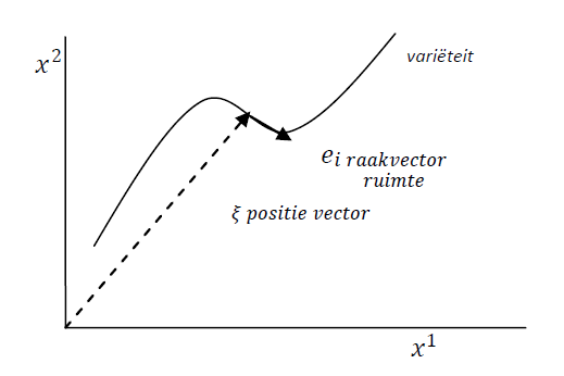
Consider a coordinate system \( x^{i} \) with an associated position vector \( \boldsymbol{\xi}(x^{i}) \), pronounced “ksi,” which represents a spatial manifold. We define the basis vectors in the tangent space as the partial derivatives of \( \boldsymbol{\xi} \):
The derivative of this basis vector with respect to another coordinate \( x^{j} \) indicates how the direction of the basis vector changes in space:
This second derivative can be expressed as a linear combination of the basis vectors themselves:
Here, \( \Gamma^{k}{}_{ij} \) is the Christoffel symbol of the second kind. This object describes how the basis vectors change, and thus the curvature of space. If this derivative is zero, the direction of the basis vector does not change and the space is flat.
2.5.1.1 Vectorial Interpretation of Directional Change
The basis vectors \( e_{i} \) belong to the tangent space at a point of the manifold. The derivative from equation (\ref{eq:R251}) tells us how this basis changes in the direction of \( x^{j} \). If \( \partial e_{i} / \partial x^{j} \neq 0 \), the space is curved.
Written out fully, equation (\ref{eq:R251}) takes the form
From here on, we omit the vector notation for \( e_{i} \) for readability.
2.5.1.2 Derivation of the Christoffel Symbol
Using the duality of basis vectors, we take the inner product with the dual basis vector \( e^{k} \):
By multiplying both sides of equation (\ref{eq:R251}) with \( e^{k} \), we obtain
This provides a direct definition of the Christoffel symbol.
2.5.1.3 Symmetry of the Lower Indices
Since in a smooth manifold the order of differentiation does not matter (\( \partial_{i}\partial_{j} = \partial_{j}\partial_{i} \)), it follows that
The Christoffel symbol is therefore symmetric in the lower indices: \( \Gamma^{k}{}_{ij} = \Gamma^{k}{}_{ji} \).
2.5.1.4 Derivation via Coordinate Transformation
Consider again
Substitution into (\ref{eq:R251}) yields
This expression shows that the Christoffel symbol is constructed from second derivatives of the coordinates, and thus is directly related to the geometry of space-time.
2.5.1.5 Relation to the Metric Tensor
The metric tensor \( g_{ik} \) is defined as the inner product of the basis vectors:
Using the inverse metric \( g^{ik} \), we can convert between basis vectors:
2.5.1.6 Summary
- The Christoffel symbol \(\Gamma^{k}{}_{ij}\) describes how basis vectors change in curved space.
- It plays a central role in the definition of the covariant derivative, which is discussed in the next section.
- The symmetry \(\Gamma^{k}{}_{ij} = \Gamma^{k}{}_{ji}\) follows from the commutativity of partial derivatives.
- The Christoffel symbol can be expressed both via coordinate derivatives and via the metric tensor, and is therefore fundamentally linked to the structure of space-time.
2.5.2 Covariant Derivative
The covariant derivative is an extension of the concept of the ordinary derivative in flat space. In general relativity, this derivative must be modified so that it is valid in curved space-time. Einstein required that his theory be covariant: physical laws must retain the same form in every coordinate system.
To ensure this, we define the covariant derivative \( \nabla \), which corrects the ordinary derivative with additional terms. This derivative satisfies
which defines the unique torsion-free, metric-compatible connection (Levi-Civita connection).
2.5.2.1 Metric and Derivatives
We start with the metric tensor (\ref{eq:R57})
Take the ordinary derivative with respect to \( x^s \):
Using the previously derived symmetry (see equation (\ref{eq:R51})), we can write:
Bringing these terms to one side of the equation, we obtain:
2.5.2.2 Definition of the Covariant Derivative
This relation motivates the definition of the covariant derivative of the metric:
We now express the tangent space derivatives in terms of Christoffel symbols. From the previous section we know:
Thus equation (\ref{eq:R61}) becomes:
Here we obtain the covariant derivative of the metric tensor, expressed in the ordinary derivative, corrected by two terms that are products of the metric tensor and the corresponding Christoffel symbol:
2.5.2.3 Cyclic Permutation
By applying the same logic to permutations of the indices, we obtain:
We now perform the following operation: (\ref{eq:R66})+(\ref{eq:R65})-(\ref{eq:R64}), taking into account the symmetry as stated in equation (\ref{eq:R51}), namely \(\Gamma^i{}_{jk} = \Gamma^i{}_{kj}\), yielding:
2.5.2.4 Christoffel Symbol via Metric
We isolate \(\Gamma^t{}_{nm}\) by multiplying with the inverse metric \(g^{st}\):
This expression gives the Christoffel symbols as a function of the metric tensor and its first derivatives.
2.5.2.5 Remarks
2.5.2.5.1 Covariance of the Metric
We confirm that the covariant derivative of the metric is indeed zero (see equation (\ref{eq:R58})):
Using: \(A_\mu = g_{\mu\nu} A^\nu\) and the Leibniz rule (product rule):
Both (73) and (74) must yield the same result, so:
Then: \(A^\nu \nabla_\rho g_{\mu\nu} = 0\). Since \(A^\nu \neq 0\), it follows that \(\nabla_\rho g_{\mu\nu} = 0\).
From this it follows that the covariant derivative of the metric is zero, which is a fundamental property of the Levi-Civita connection.
2.5.2.5.2 Transformation Rule of Vector Components
Consider a vector: \(\mathbf{V} = V^m \mathbf{e}_m\).
The component in the direction of the n-axis is:
As we know: \(g_{mn} = \mathbf{e}_m \cdot \mathbf{e}_n = g_{nm}\). Thus:
Conversely, via the inverse metric: \(g_{nm} = \frac{1}{g^{mn}}\),
2.5.2.6 Covariant Derivative of a Contravariant Vector
We now want to compute the covariant derivative of a contravariant vector field \(V^m\). In flat space, this would simply be the ordinary partial derivative. In curved space-time, however, we must take into account that the basis vectors themselves may vary from point to point.
2.5.2.6.1 Starting Point: Vector in Component Form
We consider the vector \(\mathbf{V}\) as a linear combination of basis vectors \(\mathbf{e}_m\):
The derivative of \(\mathbf{V}\) with respect to a coordinate \(x^l\) is:
2.5.2.6.2 Connection with the Christoffel Symbol
From earlier work (equation (\ref{eq:R251})) we know that the derivative of the basis vector is expressed via the Christoffel symbol:
Substitution into equation (\ref{eq:R77})) gives:
The sum over the indices m and k uses Einstein notation. We may rename dummy indices (see note below), and rewrite the second term by m → γ and k → m:
2.5.2.6.3 Definition of the Covariant Derivative
This directly yields the definition of the covariant derivative of the contravariant vector \(V^m\):
The extra term (involving the Christoffel symbol) corrects for the fact that the basis vectors themselves change in curved space. As a result, the covariant derivative \(\nabla_l V^m\) is tensorial in nature and transforms correctly under coordinate transformations.
2.5.2.6.4 Note: Dummy Indices
In Einstein notation, we are free to choose how to name the dummy index, as long as it is summed over in the product. For example:
Whether we call the index \(\mu\), \(\gamma\), or \(k\) does not affect the final result. The index merely serves as a placeholder for summation over dimensions.
2.5.2.6.5 Summary
- The covariant derivative of a contravariant vector \(V^m\) is:
\begin{align} \nabla_l V^m = \frac{\partial V^m}{\partial x^l} + \Gamma^m{}_{l\gamma} V^\gamma \end{align}
- This formula corrects the ordinary derivative with a term that reflects the curvature of space-time via the Christoffel symbol.
- The result is a tensor of the same rank as the original vector.
2.5.2.7 Covariant Derivative of a Covariant Vector
We now examine how the covariant derivative works for a covariant vector \(B_\mu\). We make use of the scalar product of a contravariant vector \(A^\mu\) and a covariant vector \(B_\mu\), and then apply the differentiation rules.
2.5.2.7.1 Starting Point: Product Rule on a Scalar Quantity
Consider the scalar product \(A^\mu B_\mu\). The covariant derivative of this product is
Substitute the expression for \(\nabla_\alpha A^\mu\) from earlier work:
Thus equation (\ref{eq:R85}) becomes:
2.5.2.7.2 Property of Scalars
Since the scalar product \(A^\mu B_\mu\) is a scalar, the covariant derivative equals the ordinary derivative:
2.5.2.7.3 Comparison of Both Expressions
By comparing the right-hand sides of (\ref{eq:R87}) and (\ref{eq:R88}):
We now rewrite the indices in the second terms on both sides to simplify the expression. Rename \(\mu \to \sigma\) and \(\nu \to \mu\) in the last term on the right-hand side. This yields:
Since this equation must hold for any \(A^\mu\), it follows that:
2.5.2.7.4 Definition
This is the covariant derivative of a covariant vector \(B_\mu\). The formula is analogous to that of contravariant vectors, but the Christoffel symbol now appears with a minus sign and with a different index position:
- For \(V^m\): \(\nabla_l V^m = \frac{\partial V^m}{\partial x^l} + \Gamma^m{}_{l\gamma} V^\gamma\)
- For \(B_\mu\): \(\nabla_\alpha B_\mu = \frac{\partial B_\mu}{\partial x^\alpha} - \Gamma^\sigma{}_{\alpha\mu} B_\sigma\)
2.5.2.7.5 Summary
- The covariant derivative of a covariant vector \(B_\mu\) is:
\begin{align} \nabla_\alpha B_\mu = \frac{\partial B_\mu}{\partial x^\alpha} - \Gamma^\sigma{}_{\alpha\mu} B_\sigma \end{align}
- The second term corrects for the change of the basis vectors in curved space.
- This definition ensures that the derivative transforms as a tensor.
2.5.3 Relation to Tensors
In this section, we investigate how a tensor constructed from the derivative of a covariant vector \(V_m\) behaves under a coordinate transformation. We show that the ordinary derivative of a vector does not yield a tensor, and that the covariant derivative is required to maintain a tensorial relation.
2.5.3.1 Transformation of a Derivative
Consider the following definition of a rank-2 tensor in the x-coordinate system:
In another coordinate system y, we write:
We now investigate whether \(T_{mn} (x)\) actually behaves as a tensor, i.e. whether equation (\ref{eq:R97}) corresponds to the transformed form of (\ref{eq:R96}).
2.5.3.2 Expected Tensor Transformation
The standard transformation formula for a covariant tensor is:
Now substitute \(T_{rs}(x) = \frac{\partial V_r (x)}{\partial x^s}\):
Note that: \(\frac{\partial V_r (x)}{\partial x^s} = \frac{\partial V_r (x)}{\partial y^n} \cdot \frac{\partial y^n}{\partial x^s}\) via the chain rule.
But the equation simplifies by directly considering:
We now want to show that: \(\frac{\partial V_m (y)}{\partial y^n} \neq T_{mn} (y)\).
2.5.3.3 Calculation of \(\frac{\partial V_m (y)}{\partial y^n}\)
Use the transformation of vector components: \(V_m (y) = \frac{\partial x^r}{\partial y^m} V_r (x)\).
Then:
Apply the product rule:
Then use the inverse transformation:
Substituting into (\ref{eq:R99}):
2.5.3.4 Relation to Christoffel Symbols
Recall that (see earlier derivation of the Christoffel symbol):
Substitution into (\ref{eq:R101}) gives:
Rearranging gives:
Thus: \(T_{mn} (y) \neq \frac{\partial V_m (y)}{\partial y^n}\).
2.5.3.5 Covariant Derivative of \(V_m\)
According to the above result:
And this is exactly the covariant derivative of the covariant vector \(V_m\) (see 2.5.2.7.4):
2.5.3.6 Conclusion
- The ordinary derivative \(\frac{\partial V_m^x}{\partial x^n}\) is not a tensor.
- Only after correction with the Christoffel symbol does a quantity arise that behaves as a tensor under coordinate transformations.
- The correct tensorial version is the covariant derivative: \(T_{mn} = \nabla_n V_m\).
2.5.3.7 Covariant Differentiation of a Covariant Tensor
2.5.3.7.1 Starting Point
Consider a tensor \(T_{\mu\nu}\), constructed as the product of two covariant vectors \(A_\mu\) and \(B_\nu\):
We now take the covariant derivative of this tensor with respect to \(x^\alpha\):
Using the product rule:
Now use the definition of the covariant derivative of a covariant vector (see section 2.5.2.7):
Substitute these into (112):
Further expand this:
2.5.3.7.2 Final Formula
Since \(T_{\mu\nu} = A_\mu B_\nu\), we finally obtain:
2.5.3.7.3 Summary
The covariant derivative of a covariant tensor \(T_{\mu\nu}\) consists of:
- the ordinary derivative \(\frac{\partial T_{\mu\nu}}{\partial x^\alpha}\),
- and two correction terms with Christoffel symbols, one for each index of the tensor.
This ensures that \(\nabla_\alpha T_{\mu\nu}\) behaves as a tensor under coordinate transformations.
2.5.3.8 Covariant Differentiation of a Contravariant Tensor
We now further extend the concept of covariant differentiation to a rank-2 contravariant tensor. This tensor has two upper indices and transforms differently from a covariant tensor. We again follow the product rule and apply the known covariant derivative formulas.
2.5.3.8.1 Starting Point
Consider a contravariant tensor \(T^{\mu\nu}\) as the product of two contravariant vectors:
The covariant derivative of \(T^{\mu\nu}\) with respect to \(x^\alpha\) is then:
Now use the formula for the covariant derivative of a contravariant vector (see section 2.5.2.6.3):
Substitution into (112) gives:
Rewrite this as:
2.5.3.8.2 Final Formula
Since \(T^{\mu\nu} = A^\mu B^\nu\), we obtain:
2.5.3.8.3 Summary
The covariant derivative of a contravariant tensor \(T^{\mu\nu}\) consists of:
- the ordinary derivative \(\frac{\partial T^{\mu\nu}}{\partial x^\alpha}\),
- and two correction terms with Christoffel symbols, one for each upper index.
The order of indices in the Christoffel symbol is important: the first (upper) index indicates which tensor index is being modified, while the two lower indices arise from the derivative.
2.5.3.9 Covariant Differentiation of a Mixed Tensor
We now consider how the covariant derivative is applied to a mixed tensor, a tensor that has both a contravariant and a covariant index.
2.5.3.9.1 Starting Point
Consider the mixed tensor \(T^\mu{}_\nu\), defined as the product of a contravariant vector \(A^\mu\) and a covariant vector \(B_\nu\):
The covariant derivative of \(T^\mu{}_\nu\) with respect to \(x^\alpha\) is:
2.5.3.9.2 Use of Covariant Derivatives
Replace the derivatives by their known expressions:
Substitute these into (\ref{eq:R125}):
Rewrite this as:
2.5.3.9.3 Final Formula
Since \(T^\mu{}_\nu = A^\mu B_\nu\), it follows that:
2.5.4 Key Points and Intuition
- Christoffel symbols \(\Gamma^\mu{}_{\nu\rho}\) describe how basis vectors change from point to point in curved space; they are constructed from the metric and its derivatives and are not tensors themselves.
- In flat space all \(\Gamma^\mu{}_{\nu\rho} = 0\); in curved space they are not, and this difference determines, among other things, parallel transport and geodesics.
- The covariant derivative corrects the ordinary derivative with terms in \(\Gamma^\mu{}_{\nu\rho}\), ensuring that the result behaves as a tensor.
- The Levi-Civita connection is torsion-free and metric-compatible \(\nabla_\alpha g_{\mu\nu} = 0\), and is therefore unique.
Intuitive
Think of walking on a sphere with an arrow in your hand: on a flat plane the arrow keeps pointing in the same direction, but on a sphere it rotates relative to the surface. That "inevitable" rotation is measured by the Christoffel symbols; the covariant derivative corrects for this rotation so that "straight ahead" retains meaning in curved geometry.
Summary overview:
| Concept | Meaning |
|---|---|
| \(\Gamma^i{}_{jk}\) | Compensation term in differentiation in curved space |
| Covariant derivative | Derivative that is "coordinate-free" and tensorial |
| \(\nabla_j V^i\) | Ordinary derivative + correction via \(\Gamma^i{}_{jk}\) |
| Geometric meaning | Parallel transport, curvature, and directional change in curved space |
2.6 Geodesic Equation and Christoffel Symbols
As discussed earlier, Einstein sought to formulate the geometry of space-time in such a way that a freely falling object experiences no force, but instead follows a "straight line" in curved space-time. Such a path is called a geodesic.
In this context, the acceleration of the four-position of the object is zero. In local free fall, the object therefore follows:
Here, \(\tau\) is the proper time, measured by an observer in a freely falling coordinate system. The origin of this system "surrenders" to gravity and follows exactly the path of the freely falling object. A geodesic is the shortest path (in proper time) between two points, given a specific space-time metric.
2.6.1 Explanation of Terms
2.6.1.1 Local (Freely Falling) Frame \(\xi^\alpha\)
This is a coordinate system defined locally in space-time. It is "freely falling" because the axes of this system behave like a particle in free fall, meaning that no non-gravitational forces act on it at that moment. On a very small scale (and approximately), the laws of physics in this system can be simplified, similar to the local laws in an inertial (straight-line, constant velocity) frame.
2.6.1.2 General Curved Coordinate System \(x^\mu\)
This is a global coordinate system describing the entire space-time, which is generally curved due to mass and energy. The coordinates \(x^\mu\) may be arbitrary coordinates used to specify points in curved space-time, without restriction to a local inertial frame.
2.6.1.3 The Relation Between the Two
The statement asserts that there exists a local transformation between these two systems, similar to a Lorentz transformation, defining the relation between the local freely falling coordinates \(\xi^\alpha\) and the general coordinates \(x^\mu\).
2.6.1.4 Meaning in Physics
In general relativity, this concept expresses that in curved space-time, one can always define a locally "flat" coordinate system at each point. In this local "free-fall" frame, the laws of physics appear the same as in a special relativistic inertial frame, simplifying the local physics. This is crucial for understanding the local effects of gravity: gravity is the manifestation of the curvature of space-time itself, and in a locally freely falling frame, this curvature can be neglected.
2.6.1.5 Derivation via Coordinate Transformation
Let \(\xi^\alpha\) be the coordinates in the local (freely falling) frame, while \(x^\mu\) are the coordinates in a general curved coordinate system. Then:
The first derivative becomes:
The second derivative:
Since \(\frac{d^2 \xi^\alpha}{d\tau^2} = 0\) for a freely falling object, it follows that:
To return to the x-coordinates, we multiply both sides by \(\frac{\partial x^\beta}{\partial \xi^\alpha}\):
Here: \(\frac{\partial \xi^\alpha}{\partial x^\mu} \frac{\partial x^\beta}{\partial \xi^\alpha} = \frac{\partial x^\beta}{\partial x^\mu} = \delta^\beta_\mu\) (the Kronecker delta).
Thus:
Recognize here the Christoffel symbol:
This yields the geodesic equation:
2.6.2 Result and Interpretation
The second derivative \(\frac{d^2 x^\beta}{d\tau^2}\) is thus compensated by the Christoffel term. When there is no gravity (i.e. flat space-time), all \(\Gamma^\beta{}_{\mu\nu} = 0\), and the object follows a straight line: \(\frac{d^2 x^\beta}{d\tau^2} = 0\).
The geodesic equation describes the path of a freely falling particle in curved space-time, i.e. the path of shortest distance in 4D space-time.
The relation between acceleration in the local free-fall frame and in the general coordinate system is:
For an object on a geodesic trajectory, the acceleration in the local frame is zero:
Or, written differently:
Here, the Christoffel symbol encodes the relation between the moving frame \(\xi^\alpha\) and the "rest" frame \(x^\beta\):
Remark 1: Affine Parameter
For massless particles such as photons, \(\tau = 0\), making proper time unsuitable. Therefore, we use an affine parameter \(\lambda\), so that the geodesic equation becomes:
The parameter \(\lambda\) often disappears in the final physical expressions, making it convenient to use.
Remark 2: Speed of Light \(c\)
In much of the literature, \(c = 1\) is chosen for simplicity. In this document, however, we keep the speed of light \(c\) explicit in the formulas. This makes it easier to check dimensions and increases the transparency of the calculations.
2.6.3 Key Points and Intuition
- Geodesics are the "straightest" possible lines in curved space-time, think of the shortest path between two points on a sphere.
- In general relativity, geodesics describe the path followed by a freely moving particle under the influence of gravity (but without other forces).
- The geodesic equation is:
\begin{align} \frac{d^2 x^\mu}{d\tau^2} + \Gamma^\mu{}_{\nu\rho} \frac{dx^\nu}{d\tau} \frac{dx^\rho}{d\tau} = 0 \end{align}
- This is a second-order differential equation that determines the trajectory in terms of the Christoffel symbols \(\Gamma^\mu{}_{\nu\rho}\).
- The equation shows that the curvature of space-time (via \(\Gamma\)) determines the acceleration of the path, without external force.
Intuitive
Imagine letting an arrow roll over a sphere without touching it:
- The arrow follows the "straightest" path on the sphere, not a straight line in the usual sense, but a great circle such as the equator or a meridian.
- This path is called a geodesic.
In relativity:
- If you drop an apple, it does not follow a curved path due to a force, but a geodesic in curved space-time, the curvature of the Earth determines the trajectory.
- The Christoffel symbols in the equation indicate how the path "deviates from straight," depending on the geometry.
Think of a GPS that adjusts its route depending on the curvature of the terrain. That "correction" is the role of \(\Gamma^\mu{}_{\nu\rho}\).
Table overview:
| Quantity | Meaning |
|---|---|
| \(x^\mu(\tau)\) | Coordinates of the particle as a function of proper time |
| \(\frac{d^2 x^\mu}{d\tau^2}\) | Acceleration along the worldline |
| \(\Gamma^\mu{}_{\nu\rho}\) | "Deflection coefficient" due to space-time curvature |
| Geodesic equation | Path without external forces: pure gravity |
2.7 Christoffel Symbols Expressed in Terms of the Metric Tensor
As discussed earlier, the metric tensor \(g_{\mu\nu}\) contains all information about the curvature and geometry of space-time. In this section, we will show how the Christoffel symbol \(\Gamma^\beta{}_{\mu\nu}\) can be expressed entirely in terms of the metric tensor and its derivatives.
2.7.1 Conditions and Definitions
We start from the following standard forms:
- Metric tensor (from local flat space):
\begin{align} g_{\mu\nu} = \eta_{\alpha\beta} \frac{\partial \xi^\alpha}{\partial x^\mu} \frac{\partial \xi^\beta}{\partial x^\nu} \end{align}where \(\eta_{\alpha\beta} = \text{diag}(1,-1,-1,-1)\) is the Minkowski metric (see also Chapter 5.6.1).
- Christoffel symbol (via transformation):
\begin{align} \Gamma^\beta{}_{\mu\nu} = \frac{\partial x^\beta}{\partial \xi^\lambda} \frac{\partial^2 \xi^\lambda}{\partial x^\mu \partial x^\nu} \end{align}
2.7.2 Transformation via Chain Rule
We begin by rewriting the metric tensor in a slightly different form \( g_{\alpha\mu} \):
by symmetry ⟹
Replace the dummy index \( \alpha \) with \( \sigma \):
Replace the index \( \nu \) with \( \alpha \):
We now rewrite the Christoffel symbol by multiplying each part of the equation by the partial derivative of \( \xi^{\sigma} \) with respect to \( x^{\beta} \):
Or:
i.e. \( \delta_{\lambda\sigma} = 1 \) if \( \sigma = \lambda \) and \( = 0 \) if \( \sigma \ne \lambda \)
Thus together with (\ref{eq:R154}) this becomes:
If \( \sigma = \lambda \), we replace \( \lambda \) by \( \sigma \):
Thus from (\ref{eq:R153}):
Using (\ref{eq:R157}) we can derive:
We now rewrite:
We know from above:
Thus:
Perform cyclic permutations:
Now take (\ref{eq:R163})+(\ref{eq:R164})-(\ref{eq:R165}):
By symmetry:
Isolating the Christoffel symbol:
Replace \( \rho \) by \( \beta \):
Usually:
Thus in compact notation:
2.7.3 Summary
The Christoffel symbols are fully expressed in terms of the metric tensor \(g_{\mu\nu}\) and its first derivatives:
Or in short notation:
2.7.4 Key Points and Intuition
- Christoffel symbols \(\Gamma^\lambda{}_{\mu\nu}\) can be fully computed from the metric tensor \(g_{\mu\nu}\).
- The explicit formula is:
\begin{align} \Gamma^\lambda{}_{\mu\nu} = \frac{1}{2} g^{\lambda\rho} \left( \partial_\mu g_{\rho\nu} + \partial_\nu g_{\rho\mu} - \partial_\rho g_{\mu\nu} \right) \end{align}
- The Christoffel symbols indicate how coordinate systems are locally curved, and thus how vectors and trajectories behave.
- The symmetry \(\Gamma^\lambda{}_{\mu\nu} = \Gamma^\lambda{}_{\nu\mu}\) is preserved as long as the metric is symmetric (which it always is).
- This relation forms the bridge between geometry and dynamics in general relativity.
Intuitive
The metric tensor \(g_{\mu\nu}\) tells you how to measure distances in a space (e.g. how "far" something is in curved coordinates).
But: if you move through a landscape and want to know how the direction of an arrow changes as you move forward, you need more than just distances, you must know how the measuring rods themselves change. That is exactly what the Christoffel symbols do.
You can think of it this way:
- The metric tells you what is straight at a point.
- The Christoffel symbols tell you how "straight" changes as you move.
You do not need to measure the change of basis vectors separately, you can compute it entirely from the metric itself!
Table overview:
| Quantity | Meaning |
|---|---|
| \(g_{\mu\nu}\) | Determines local distance and angle |
| \(\partial_\sigma g_{\mu\nu}\) | How the distance definition changes as you move |
| \(\Gamma^\lambda{}_{\mu\nu}\) | How basis vectors change, determines deviation from "straight" |
| Formula | Derivatives of the metric combined with the inverse metric |
2.8 Geodesic Equation and its Newtonian Limit
Newtonian gravity describes how matter generates a gravitational potential Φ, and how, according to Newton’s second law, that potential leads to an acceleration:
Here Φ is the gravitational potential, and ∇ is the Euclidean gradient operator
Here \( \mathbf{e}_x, \mathbf{e}_y, \mathbf{e}_z \) are the unit vectors along the respective axes. This description is accurate at low velocities, weak fields, and in a static regime. We will now show that the geodesic equation of general relativity reduces to the Newtonian gravitational equation in this limit.
2.8.1 Assumptions for the Newtonian Limit
- The particle moves slowly compared to the speed of light.
- The gravitational field is weak.
- The field is static, i.e. it does not change with time.
2.8.2 Starting Point: the Geodesic Equation
The geodesic equation describes the worldline of a particle influenced only by gravity. We will now show that in the context of the Newtonian limit, the geodesic equation reduces to the Newtonian equation of gravity.
From the previous section we know that the geodesic equations, with proper time as the parameter of the worldline, are given by:
The second term involves a sum over \( \mu \) and \( \nu \) over all indices, resulting in 16 terms. Because the particle moves very slowly relative to the speed of light, the time component (the 0th component of the particle’s vector) dominates over the spatial components. We then arrive at the following approximation:
The only term that remains after approximation is the time component, i.e. \( \Gamma^{\beta}_{00} \) with \( \mu = \nu = 0 \). This gives:
For describing four-dimensional space-time, Greek letters are typically used for indices, but when considering only three-dimensional space, it is customary to use Latin letters. Therefore, \( \beta \) is replaced by \( i \) (i = x, y, z), resulting in:
2.8.3 Approximation of the Christoffel Symbol
From the chapter Christoffel symbols expressed in terms of the Metric Tensor (2.7), it follows that the Christoffel symbol can be calculated with respect to the components of a given metric where \( x^0 \equiv \tau \):
so that the Christoffel symbol simplifies to:
2.8.4 Weak-Field Approximation
If the gravitational field is sufficiently weak, spacetime will only be slightly distorted relative to the gravity-free Minkowski spacetime of Special Relativity. The spacetime metric can then be considered as a small perturbation of the Minkowski metric \( \eta_{\mu\nu} \):
For \( g_{00} \) we then have:
Thus, from (\ref{eq:R188}) and (\ref{eq:R192}), equation (\ref{eq:R185}) becomes:
By defining \( g_{ij} = \eta_{ij} - h_{ij} \), we find that
We then obtain:
But since \( \eta_{ij} \) is nonzero for \( j = i \), we have \( \eta_{ii} = -1 \) (where i refers to spatial components), so:
We now transform the derivative on the left-hand side from \( \tau \) to \( t \), as follows:
First, in the above equation, replace i with 0, so that \( x^0 = t \):
Since the gravitational field is constant:
2.8.5 Switching to Coordinate Time
We now manipulate the derivatives with respect to proper time (\( \tau \)):
As shown above in (\ref{eq:R200}), we have:
It follows that:
In general:
2.8.6 Equation in Newtonian Form
In vector form:
where
This is another way to write the Newtonian gravitational law
2.8.7 Metric Component in Terms of the Potential
By writing the metric \(g_{00}\) as:
the direct link becomes visible between the metric tensor (component \(g_{00}\)) on the left-hand side and the gravitational potential \(\phi\) on the right-hand side.
2.8.8 Example: Calculation of \(h_{00}\) on Earth
The value of \( h_{00} \) on Earth can now be calculated to verify whether this value is negligible, meaning that the deviation from the Minkowski metric due to the gravitational field is negligible.
Or:
With:
- \( G = 6.67 \times 10^{-11} \, \text{m}^3 \cdot \text{kg}^{-1} \cdot \text{s}^{-2} \)
- \( M_{\text{earth}} \simeq 6 \times 10^{24} \, \text{kg} \quad R_{\text{earth}} \simeq 6400 \, \text{km} \)
- \( c \simeq 3 \times 10^8 \, \text{m} \cdot \text{s}^{-1} \)
We obtain:
For the Sun this is ~\(10^{-6}\) and for a white dwarf ~\(10^{-4}\), confirming that the weak-field approximation is generally valid in many realistic situations.
2.8.9 Key Points and Intuition
- In general relativity, free particles follow a geodesic in curved spacetime.
-
In the classical case (Newton), a particle follows a trajectory under the influence of gravity:
\begin{align} \mathbf{a} = -\nabla \Phi \end{align}where \( \Phi \) is the gravitational potential.
- In the weak-field approximation and for low velocities, the geodesic equation reduces to this Newtonian form.
- This requires:
-
Spacetime is only weakly curved ⟹
\begin{align} g_{\mu\nu} = \eta_{\mu\nu} + h_{\mu\nu} \end{align}
-
Only \( g_{00} \) deviates significantly from the flat Minkowski metric ⟹
\begin{align} g_{00} \approx -\left(1 + \frac{2\phi}{c^2}\right) \end{align}
-
The component \( \Gamma^{i}_{00} \) turns out to be
\begin{align} \frac{1}{2}\partial_i g_{00} \approx \partial_i \phi \end{align}which leads to Newton’s gravitational equation.
Intuition
Einstein’s theory must reproduce the same predictions as Newton’s theory in everyday situations. That is:
- If gravity is weak (e.g., near Earth),
- And velocities are much smaller than the speed of light (e.g., falling apples),
- Then the relativistic formula must reduce to the classical one.
The geodesic equation states: “a particle moves in curved spacetime, without force.” But in weak fields, that curvature can be written as a small deviation from flat spacetime. That deviation then appears as an “effective force”, exactly as Newton described it.
Thus: Newton’s gravity is a limiting case of general relativity. The apple falls, not because of a force, but because the time component \( g_{00} \) is slightly curved by the mass of the Earth.
Summary comparison table:
| Theory | Formula | Interpretation |
|---|---|---|
| Newton (classical) | \( \mathbf{a} = -\nabla \Phi \) | Acceleration due to force |
| Einstein (weak limit) | \( \frac{d^2 x^i}{dr^2} = -\Gamma^{i}_{00} \) | Deviation from straight motion due to time curvature |
| Link between both | \( \Gamma^{i}_{00} = \frac{1}{2}\partial_i g_{00} \approx \partial_i \phi \) | \( g_{00} \) encodes the potential |
2.9 Generalizing the Definition of the Metric Tensor
In the previous sections, we have seen how the geodesic equation is generalized from an inertial frame to an arbitrary coordinate system. In a similar way, we now extend the definition of the line element from flat Minkowski spacetime to a general curved spacetime, a so-called pseudo-Riemannian manifold. This structure forms the mathematical foundation of general relativity.
2.9.1 The Minkowski Line Element in a Local Inertial Frame
In a local inertial frame we use the coordinates \( \xi^\alpha \), defined as:
The Minkowski line element can be described as follows (see also Independence of the Chosen Coordinate System 2.2.2) equation (\ref{eq:R19}) and see also 5.6.1 Extended Explanation of the Metric Tensor)
The corresponding line element reads:
where \( \eta_{\alpha\beta} \) is the Minkowski metric:
2.9.2 Coordinate Transformation to a General System
We now move to an arbitrary, possibly curved coordinate system \(x^\mu\), in which the old coordinates \(\xi^\alpha\) are functions of the new ones:
The differential change \(d\xi^\alpha\) is then, via the chain rule:
Using the Einstein summation convention:
We can then rewrite the line element as:
2.9.3 Definition of the General Metric Tensor
We now define the metric tensor \(g_{\mu\nu}\) as:
So that the line element in the new system becomes:
2.9.4 Properties of the Metric Tensor
The properties of the metric tensor are:
- Symmetry:
\begin{align} g_{\mu\nu} = g_{\nu\mu} \end{align}This follows directly from the definition, since the Minkowski metric is symmetric.
- Inverse metric:
\begin{align} g^{\mu\sigma} g_{\sigma\nu} = \delta^\mu_\nu \end{align}where \(\delta^\mu_\nu\) is the Kronecker delta.
- Covariant versus contravariant:
The inverse \(g^{\mu\nu}\) is called the contravariant metric; \(g_{\mu\nu}\) is the covariant metric.
2.9.5 Importance of the Metric in Relativity
The metric tensor contains all the information about the structure of spacetime. It determines distances, angles, curvature, and thus also the behavior of objects under the influence of gravity. In the context of general relativity, gravity is nothing more than a manifestation of the curvature of spacetime. This curvature is fully described by the metric.
Therefore, the fundamental goal of general relativity is to find \(g_{\mu\nu}\), the metric, as a solution of the Einstein field equations. Once known, this tensor determines the motion of free particles, the curvature of space and time, and the interaction with energy and mass.
2.9.6 Number of Independent Components
Although \(g_{\mu\nu}\) appears at first to have 16 components (in a 4×4 matrix), it is symmetric: \(g_{\mu\nu} = g_{\nu\mu}\). Therefore, only 10 independent components remain. These ten functions of spacetime are the unknowns in Einstein’s field equations.
2.9.7 Key Points and Intuition
- The metric tensor \(g_{\mu\nu}\) defines distance in spacetime via the line element:
\begin{align} ds^2 = g_{\mu\nu} dx^\mu dx^\nu \end{align}
- This formula holds in any coordinate system, flat or curved, as long as \(g_{\mu\nu}\) is correctly adapted.
- The metric is:
- Symmetric: \(g_{\mu\nu} = g_{\nu\mu}\)
- Tensorial: transforms according to tensor transformation laws under coordinate changes.
- The metric contains all information about local geometry: distance, angle, volume, and light cones.
- In curved space, the metric is position-dependent: \(g_{\mu\nu} = g_{\mu\nu}(x)\)
- Through generalization, the metric becomes the fundamental object upon which all other geometric quantities are based (Christoffel symbols, Riemann tensor, etc.).
Intuitive
In special relativity, distance in spacetime is something like:
In general relativity, we say: spacetime itself is deformable, so that distance formula must be adapted to curvature. We do this with a metric tensor \(g_{\mu\nu}\), which at each point tells us how space and time are measured.
You can think of it as a ruler that locally changes shape depending on where you are. Sometimes a “meter” is more or less than elsewhere, and angles can become skewed, depending on the mass/energy nearby.
The generalization means that we no longer have a universal, fixed formula for distance, but a flexible field that varies from point to point, and behaves tensorially.
Table Overview
| Quantity | Meaning |
|---|---|
| \(g_{\mu\nu}(x)\) | Local measurement rule for spacetime |
| Symmetry | \(g_{\mu\nu} = g_{\nu\mu}\) |
| Tensor transformation | The metric adapts under coordinate transformations |
| Distance | \(ds^2 = g_{\mu\nu} dx^\mu dx^\nu\) |
| Special limit | \(g_{\mu\nu} = \eta_{\mu\nu}\) (Minkowski metric) |
2.10 The Riemann Curvature Tensor
The Riemann curvature tensor is one of the most important concepts in general relativity. This tensor describes how spacetime is locally curved as a result of the presence of mass and energy. It determines how vectors change under parallel transport along curved paths around a closed loop.
In flat, Euclidean space, where no gravitational effects occur, the Riemann tensor vanishes: \(R^\rho_{\sigma\mu\nu} = 0\) (in flat spacetime).
In this chapter, we derive the Riemann tensor in two ways:
- Via the commutator of two covariant derivatives
- Via the method of geodesic deviation
2.10.1 Derivation via the Commutator of Covariant Derivatives
Using the concept of parallel transport of vectors or tensors, we will derive the expression for the Riemann tensor.
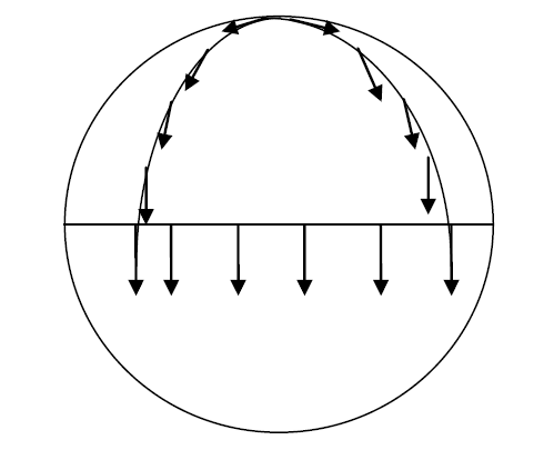
An intuitive example of curvature can be found on the surface of the Earth. Suppose we walk with a horizontally held stick from the North Pole along a meridian to the equator. There we turn 90 degrees, walk along the equator, and return via another meridian to the North Pole. Even though we keep the stick in the "same direction," it points in a different direction upon return. This difference is due to the curvature of the surface.
In a similar way, we can parallel transport a vector in an infinitesimal loop on a manifold. In flat space, the vector does not change; in curved space, it does. This difference in parallel transport is directly related to the Riemann tensor.
We define parallel transport as motion for which the covariant derivative of a vector is zero. To derive the Riemann tensor, we investigate how the result of applying two covariant derivatives depends on their order. The commutator of the covariant derivatives provides a measure of curvature.
2.10.1.1 Covariant Derivative Commutator
A commutator here refers to the difference between two operations, where one is performed in one order and the other in the opposite order. The commutator is defined as:
The commutator is therefore zero only when the order of the two operations is irrelevant.
To obtain the Riemann tensor, the covariant derivative is chosen as the operation. The commutator of two covariant derivatives measures the difference between parallel transporting a tensor first in one direction and then in the opposite direction. Thus, as a measure of the difference of the tensor along a path, the covariant derivative of the tensor is used.
In flat space, the order of covariant derivatives makes no difference, because covariant differentiation reduces to partial differentiation, and therefore the commutator must vanish. Conversely, any non-zero result from applying the commutator to covariant differentiation can be attributed to the curvature of space, and is therefore identified as the Riemann tensor.
2.10.1.2 Derivation of the Riemann Tensor
The goal is now to derive the Riemann tensor by evaluating the following commutator:
We know that the covariant derivative of \(V_a\) is given by (see equation (\ref{eq:R94}):
And that this derivative itself is a tensor. As we saw in the previous chapter:
(see equation (\ref{eq:R109}))
This means that:
Thus, the covariant derivative of a vector \((\nabla_b V_a)\) is a tensor (see equation (\ref{eq:R109})). The covariant derivative of a tensor is (see equation (\ref{eq:R118})):
This results in:
The first term on the right-hand side:
Expanded:
The second and third terms on the right-hand side:
By combining the three terms ((\ref{eq:R242}), (\ref{eq:R243}),(\ref{eq:R244}) into (\ref{eq:R240}), we obtain:
By interchanging b and c, we find:
By subtracting (\ref{eq:R246}) from (\ref{eq:R245}), the first and last terms cancel. Since the Christoffel symbol is symmetric with respect to the lower indices, we obtain:
Expanding the parentheses in the last terms and factoring the terms with \(V_d\):
From equation (\ref{eq:R251}) in the previous chapter, we know:
Therefore:
Or, combined and regrouped by explicitly factoring out the vector \(V_d\):
After interchanging d with e in the first and third terms on the right-hand side:
We define the expression in parentheses on the right-hand side as the Riemann tensor, which means that:
This is the component form of the Riemann tensor, which explicitly contains the derivatives of the Christoffel symbols and their products. This expression shows how curvature is an intrinsic geometric effect that cannot be removed by a change of coordinates.
Note: Here the commutator can be interpreted as the difference between two vectors. The magnitude of the resulting vector is the Riemann tensor.
2.10.1.3 Alternative Derivation of the Riemann Tensor via the Commutator
We consider an infinitesimal region over which a vector is transported (parallel transported) along two different paths. When the manifold is flat, the difference between the two resulting vectors would be zero. However, in the case where the manifold is intrinsically curved, this leads to a difference between the resulting vectors.
First, we move a vector \(V\) from point A via B to C. To determine the direction of motion of the vector, we take the derivative of the vector with respect to \(dx^\mu\), and then examine the change of this result with respect to \(dx^\nu\).
Next, we do the same from A via D to C, now first with respect to \(dx^\nu\) and then with respect to \(dx^\mu\). We then subtract the two results, which should lead to the Riemann tensor.
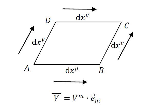
The vector \( e_m \) is the tangent vector, i.e., the derivative of the position vector or the derivative of the trajectory. If the trajectory is a straight line, then the derivative of \( e_m \) is constant; and consequently, the derivative of \( e_m \), and thus the Christoffel symbol, is zero.
First, from A to B, to determine the direction, we take the derivative (see also equation (\ref{eq:R250})):
Change the two dummy indices, \( k \) and \( m \). Then the formula can be adjusted from \( k \) to \( m \) and \( m \) to \( \gamma \):
This is the covariant derivative of the contravariant vector \( V \). And from the definition of the Christoffel symbol in the previous chapters, we know that:
Next, the change in direction from B to C with respect to \( dx^\nu \):
In the right-hand side of the equation, replace in the second term the indices \( k \) with \( m \) and \( m \) with \( \gamma \), and interchange \( k \) and \( m \) in the fifth term:
Now for the other direction, interchange \( \mu \) and \( \nu \):
Now subtract the last two equations:
The fifth-sixth, seventh-eighth, and ninth-tenth terms vanish. Therefore:
2.10.1.4 Definition of the Riemann Tensor
The expression within the parentheses is defined as the Riemann tensor:
Here, the Riemann tensor describes the degree of curvature of spacetime through the difference in parallel transport of a tensor around a closed loop.
2.10.1.5 Conclusion
This alternative derivation of the Riemann tensor via the commutator provides a way to understand how the curvature of spacetime is determined by the difference in parallel transport of tensors. The Riemann tensor is therefore a crucial tool in general relativity for describing the geometry and gravitational effects in spacetime.
2.10.2 Derivation of the Riemann Tensor via Geodesic Deviation
In the previous chapter, we presented a method to derive the Riemann tensor from the commutator of covariant derivatives, which physically corresponds to the difference between parallel transporting a vector first along one path and then along another. Another interpretation arises from the relative acceleration of nearby particles in free fall.
Imagine a cloud of particles in free fall. Let us assume that an observer travels along with one of these particles. He observes a nearby particle and measures its position in local inertial coordinates. In special relativity, this particle would move in a straight line with constant velocity, without acceleration. But what happens in a gravitational field?
As we recall from the previous chapter, a geodesic generalizes the concept of a "straight line" to curved spacetime.
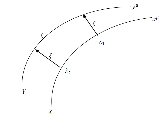
Here we will show how the evolution of the distance measured between two neighboring geodesics, also known as geodesic deviation, can indeed be related to a non-zero curvature of spacetime, or in Newtonian terms, to the presence of tidal forces. Let us therefore consider two particles following two very close geodesics.
Their respective paths can be described by the functions \( x^\mu(\tau) \) (for the reference particle) and \( y^\mu(\tau) \equiv x^\mu(\tau) + \xi^\mu(\tau) \) (for the second particle), where \( \tau \) (tau) is the proper time along the worldline of the reference particle, and where \( \xi^\mu \) denotes the deviation four-vector connecting one particle to the other at each instant \( \tau \).
Our goal in this chapter is to show that this relative acceleration is related to the Riemann tensor via the following equation:
In the case where spacetime is flat, the Riemann tensor is zero, resulting in zero relative acceleration.
Since each particle follows a geodesic, the equation of their respective coordinates is given as follows (see equation (\ref{eq:R144})):
In each of these equations, the Christoffel symbol is evaluated at the respective positions of the particles \( x \) and \( y \). Since the separation between the particles is infinitesimal, we evaluate the Christoffel symbol at the position \( y^\alpha(\tau) \) by means of a Taylor series expansion:
Approximating to first order since \( \xi \) is infinitesimal:
This can also be approximated as follows for an infinitesimal \( \Delta x \):
Assuming that \( y^\alpha(\tau) = x^\alpha(\tau) + \xi^\alpha(\tau) \), and substituting this expression into the geodesic equation for particle \( y \), we obtain:
Here, the Christoffel symbol and its first-order derivatives are now evaluated at \( x^\alpha(\tau) \).
Expanding all terms in the parentheses and neglecting second-order terms in \( \xi \), we obtain:
Since we know that the Christoffel symbol is symmetric with respect to the lower indices, these can be interchanged:
Using the geodesic equation for particle \( x \), as given (see equation (\ref{eq:R144})):
Then the first and the third terms cancel. We then obtain:
Here,
Next, we have an expression for
Replacing the dummy index \( \alpha \) by \( \sigma \) in the second term and using the definition of the Christoffel symbol, we obtain:
Thus:
Since we are still dealing with the condition that \( \xi \) is a four-vector, its derivative with respect to proper time is also a four-vector, so we can find the second absolute derivative by using the same procedure as for the first derivative.
Using the Christoffel symbols and the Taylor expansion above, and replacing \( \nu \) by \( \sigma \) in the first term, we obtain:
We can rewrite the second term, since the Christoffel symbols depend on \( \tau \) through their dependence on the position of the reference particle:
Using the geodesic equation, we can rewrite the third term, i.e., expand \( \frac{du^\mu}{d\tau} \):
Also, to obtain an expression for \(u^\nu u^\mu \xi^\sigma\) involving only \( \mu,\nu \) and \( \sigma \), we can rewrite the last term by renaming the dummy indices \( \sigma \) and \( \beta \):
Thus, finally, by substituting all terms, we can write:
Eliminating the first and the fifth terms and factoring out the common factor \(u^\nu u^\mu \xi^\sigma\), we obtain:
Since this is still a tensor equation, the quantity in parentheses is a tensor, and we can define the Riemann tensor as:
We can then rewrite the above equation in a shorter form, known as the geodesic deviation equation:
Since the only quantity in this equation that intrinsically depends on the metric is the Riemann tensor, we see that if it is identically zero, then spacetime is flat. However, if even a single component of this tensor is non-zero, then spacetime is curved.
2.10.3 Key Points and Intuition
- The Riemann tensor \(R_{\sigma\mu\nu}^{\rho}\) is the fundamental tensor that describes the curvature of spacetime.
- It can be derived via the commutator of covariant derivatives, or via the geodesic deviation equation.
- Its component form is:
\begin{align} R_{\mu\sigma\nu}^{\alpha}=\frac{d\Gamma_{\mu\nu}^{\alpha}}{dx^{\sigma}}-\frac{d\Gamma_{\mu\sigma}^{\alpha}}{dx^{\nu}}+\Gamma_{\gamma\sigma}^{\alpha}\Gamma_{\nu\mu}^{\gamma}-\Gamma_{\nu\gamma}^{\alpha}\Gamma_{\mu\sigma}^{\gamma} \end{align}
- For a geodesic curve, the following property holds:
\begin{align} 0=\frac{d^2 x^\beta}{d\tau^2}+\Gamma_{\mu\nu}^{\beta}\frac{\partial x^\mu}{\partial \tau}\frac{\partial x^\nu}{\partial \tau} \quad \text{Geodesic equation} \end{align}
- Or:
\begin{align} \frac{d^2 x^\beta}{d\tau^2}=-\Gamma_{\mu\nu}^{\beta}u^\nu u^\mu \end{align}
- Whereas for the deviation from one geodesic to an infinitesimally nearby geodesic, we have:
- A non-zero Riemann tensor implies curved spacetime and thus the presence of gravity.
- Measures the non-commutativity of applying covariant derivatives twice to a vector:
\begin{align} \left(\nabla_\mu\nabla_\nu-\nabla_\nu\nabla_\mu \right) V_\rho=R_{\sigma\mu\nu}^{\rho}V_\sigma \end{align}
The tensor can be fully expressed in terms of Christoffel symbols and their derivatives.
- In flat space, \(R_{\sigma\mu\nu}^{\rho}=0\); in curved space, it is generally non-zero.
- Curvature is locally measurable via the behavior of geodesics: if two free particles that start close together begin to deviate, this indicates curvature.
Intuitive
Imagine two rockets starting side by side in space, moving without engines (free fall), each at a slightly different position. In flat space they remain parallel, but in curved space (e.g., around a planet) they will bend toward or away from each other.
The Riemann tensor measures exactly that effect:
- How does the “direction” of a vector change when transported around a closed loop?
- If the result differs from the original vector, the space is curved.
You can compare it to carrying an arrow around a sphere: when you return, it no longer points in the same direction, curvature manifests as a change in direction.
Table overview:
| Quantity | Meaning |
|---|---|
| \(R^\rho_{\sigma\mu\nu}\) | Measures curvature via comparison of transport |
| Building blocks | Christoffel symbols + their derivatives |
| Physical meaning | Deviation between nearby geodesics |
| Zero in flat space | \(R^\rho_{\sigma\mu\nu}\) |
| Dimension | Rank-4 tensor (4 indices) |
2.11 Symmetries and Independent Components
In the previous chapters, we derived the rather complex expression for the Riemann curvature tensor—a combination of derivatives and products of Christoffel symbols, with a total of 256 (=4⁴) components in four-dimensional spacetime. In this chapter, we show that the Riemann tensor actually has only 20 independent components, fully determined by its symmetries and the second-order derivatives of the metric.
We analyze these symmetries in a Local Inertial Frame (LIF), where all Christoffel symbols vanish at the origin. However, these symmetries are not restricted to this specific frame: since tensor equations are coordinate-independent, they hold in any reference frame.
2.11.1 Definition and Reformulation
The Riemann tensor is generally defined as:
Knowing that all Christoffel symbols, \(\Gamma = 0\), vanish at the origin of the Local Inertial Frame, this reduces to:
By applying the contraction mechanism, we can rewrite the Riemann tensor with all indices lowered:
The Christoffel symbols can be expressed in terms of the metric:
So that we can write:
The second term is zero because the Christoffel symbols vanish at the origin of the local inertial frame, as stated above:
With this result and from equation (\ref{eq:R328}) it follows:
Interchanging the indices \(\mu\) and \(\nu\) leads to the second term in the expression of the Riemann tensor:
The middle terms cancel after subtracting the last two expressions, resulting in:
Multiplying by \(-1\):
Interchanging \(\mu\) and \(\nu\) in (2):
Thus, from (\ref{eq:R333}) and (\ref{eq:R334}) we obtain:
Note that this equation is only valid at the origin of the Local Inertial Frame. However, since these are tensor equations and, as we know, if they hold in one reference frame, they hold in every reference frame.
Now we will show in a similar way that the Riemann tensor is antisymmetric under interchange of the first two indices:
If we interchange the first and third indices (\(\alpha \leftrightarrow \mu\)), and also the second and fourth (\(\beta \leftrightarrow \nu\)), we obtain:
If we cyclically permute the last three indices \(\beta,\mu,\nu\) and add the three terms, we obtain:
2.11.2 Symmetry Properties
From the above expression, we can derive the following symmetries of the Riemann tensor:
-
Antisymmetry in the last two indices:
\begin{align} R_{\alpha\beta\mu\nu} = - R_{\alpha\beta\nu\mu} \end{align} -
Antisymmetry in the first two indices:
\begin{align} R_{\alpha\beta\mu\nu} = - R_{\beta\alpha\mu\nu} \end{align} -
Symmetry under interchange of index pairs:
\begin{align} R_{\alpha\beta\mu\nu} = R_{\mu\nu\alpha\beta} \end{align} -
The first Bianchi identity (cyclic symmetry):
\begin{align} R_{\alpha\beta\mu\nu} + R_{\alpha\nu\beta\mu} + R_{\alpha\mu\nu\beta} = 0 \end{align}
Or represented as:
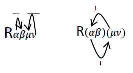
Antisymmetry means that the tensor changes sign under interchange of these indices, which is related to the orientation of loop integration in parallel transport.
2.11.3 Number of Independent Components
In four-dimensional spacetime, with four values per index, an arbitrary (0,4)-tensor would have 256 components. Due to the above symmetries, this number is drastically reduced:
- Due to antisymmetry in \( \alpha\beta \) and \( \mu\nu \): from \( 4^4 = 256 \) to \( 4^2 \times 4^2 = 6 \times 6 = 36 \)
- Symmetry between the pairs: \( 36 \rightarrow \dfrac{6 \times (6+1)}{2} = 21 \)
- Bianchi identity: further reduces the number to 20 independent components
2.11.4 Key Points and Intuition
-
The Riemann tensor \( R_{\rho\sigma\mu\nu} \) possesses several symmetries, which strongly restrict the number of independent components:
- Antisymmetry in the last two indices:
\begin{align} R_{\rho\sigma\mu\nu} = - R_{\rho\sigma\nu\mu} \end{align} - Antisymmetry in the first two indices:
\begin{align} R_{\rho\sigma\mu\nu} = - R_{\sigma\rho\mu\nu} \end{align} - Symmetry under interchange of index pairs:
\begin{align} R_{\rho\sigma\mu\nu} = R_{\mu\nu\rho\sigma} \end{align} - Bianchi identity (cyclic property):
\begin{align} R_{\rho\sigma\mu\nu} + R_{\rho\mu\nu\sigma} + R_{\rho\nu\sigma\mu} = 0 \end{align}
- Antisymmetry in the last two indices:
- Due to these symmetries, the Riemann tensor in 4D has only 20 independent components, not 256.
Thus, although the original expression of the Riemann tensor appears complex, its rich symmetry structure means it is fully determined by only 20 independent components. These components represent all possible forms of curvature in four-dimensional spacetime and therefore form the core of the geometric description of gravity in general relativity.
Intuition
Imagine a cube with 4 index positions, in principle there would be \( 4 \times 4 \times 4 \times 4 = 256 \) components. But due to symmetries such as:
- “if you swap these two indices, only the sign changes”
- “if you swap the pairs, it remains the same”
it turns out that many of those 256 values are related. Think of a painting with mirror symmetry: if you know one half, you also know what must appear on the other side. The same idea applies to the structure of the Riemann tensor.
These properties are not accidental, but arise from the way the tensor is derived from the metric and its derivatives.
Table overview:
| Symmetry | Explanation |
|---|---|
| \( R_{\rho\sigma\mu\nu} = - R_{\rho\sigma\nu\mu} \) | Antisymmetry in last two indices |
| \( R_{\rho\sigma\mu\nu} = - R_{\sigma\rho\mu\nu} \) | Antisymmetry in first two indices |
| \( R_{\rho\sigma\mu\nu} = R_{\mu\nu\rho\sigma} \) | Interchange of index pairs |
| Bianchi identity | Linear relation between permutations of indices |
| Total in 4D | 20 independent components |
2.12 Bianchi Identity and Ricci Tensor
The Bianchi identity plays a crucial role in deriving Einstein’s field equations. Although the Riemann curvature tensor itself does not appear directly in these equations, we can derive two other important curvature quantities from it, via contraction: the Ricci tensor and the Ricci scalar.
In this chapter, we will introduce these three fundamental objects and explain their relationships, starting with the derivation of the Bianchi identity.
2.12.1 Bianchi Identity
The Bianchi identity is given by:
From the previous chapter 2.11 Symmetries and Independent Components, we know that at the origin of a Local Inertial Frame the Riemann tensor can be written as:
Since the Christoffel symbols vanish at the origin of this frame, the covariant derivative reduces there to the ordinary derivative:
Substituting the expression for the Riemann tensor yields:
By cyclically permuting the derivative index with the last two indices \(\mu,\nu\) of the tensor, we obtain:
Adding these three equations and using the commutativity of partial derivatives, we see that the terms cancel pairwise, yielding the Bianchi identity:
This Bianchi identity is a tensor equation that holds universally, in any coordinate system.
2.12.2 Key Points and Intuition
-
The Bianchi identity is a fundamental identity of the Riemann tensor:
\begin{align}\nabla_\lambda R^\rho_{\sigma\mu\nu} + \nabla_\mu R^\rho_{\sigma\nu\lambda} + \nabla_\nu R^\rho_{\sigma\lambda\mu} = 0\end{align} -
By contraction, this leads to the so-called contracted Bianchi identity:
\begin{align}\nabla^\mu \left(R_{\mu\nu} - \tfrac{1}{2} g_{\mu\nu} R\right) = 0\end{align} - This contracted version is crucial for the consistency of the Einstein field equations.
-
It implies that the derivative of the tensor
\(G_{\mu\nu} = R_{\mu\nu} - \tfrac{1}{2} g_{\mu\nu} R\) vanishes:
\begin{align}\nabla^\mu G_{\mu\nu} = 0\end{align} - This corresponds to the conservation of energy and momentum in curved spacetime.
Intuitive
The Riemann tensor is not just an arbitrary object—it must satisfy deeper structural rules. The Bianchi identity is such a rule: a kind of internal consistency condition of spacetime curvature.
When working with vectors, one might say: “the divergence of a force is zero if there are no sources.” With tensors, a similar idea applies: the structure of curvature is organized in such a way that certain combinations always vanish—and this implies, among other things, that the Einstein equations do not allow energy to appear out of nothing.
The contracted Bianchi identity is essential because it guarantees that the Einstein tensor \(G_{\mu\nu}\) automatically satisfies a conservation law: energy and momentum are conserved in any curved spacetime.
Table overview:
| Quantity | Meaning |
|---|---|
| Bianchi identity | Structural symmetry of the Riemann tensor |
| Contracted Bianchi identity | Implies \(\nabla^\mu G_{\mu\nu} = 0\) |
| Einstein tensor \(G_{\mu\nu}\) | \(G_{\mu\nu} = R_{\mu\nu} - \tfrac{1}{2} g_{\mu\nu} R\) |
| Physical meaning | Ensures conservation of energy and momentum in curved spacetime |
2.12.3 The Ricci Tensor
In the next chapter, we will deal with the energy-momentum tensor. This tensor is a rank-2 tensor. For this reason, we must reduce the rank-4 Riemann tensor to a rank-2 tensor, which is called the Ricci tensor. This can be done by contracting the covariant Riemann tensor with a rank-2 contravariant metric tensor, sharing two common indices. This process is called contraction.
By contracting the first and third indices of the Riemann tensor, we obtain the Ricci tensor:
The Ricci tensor is symmetric:
2.12.4 The Ricci Scalar
By contracting the Ricci tensor with the metric tensor with matching indices, the Ricci tensor is further contracted, resulting in the Ricci scalar:
This scalar curvature \(R\) is the trace of the Ricci tensor.
These tensors, the Ricci tensor and Ricci scalar,together with the metric \(g_{\mu\nu}\), form the building blocks of Einstein’s field equations. The Bianchi identity further guarantees the conservation laws that follow from these equations.
2.12.5 Key Points and Intuition
-
The Ricci tensor \(R_{\mu\nu}\) is a contraction of the Riemann tensor:
\begin{align} R_{\mu\nu} = R^{\lambda}_{\mu\lambda\nu} \end{align} - It contains information about how volumes change in curved spacetime (think of expansion or contraction of bundles of geodesics).
-
The Ricci scalar \(R\) is a further contraction:
\begin{align} R = g^{\mu\nu} R_{\mu\nu} \end{align} - These quantities are coordinate-independent and form the basis of the Einstein field equations.
- While the Riemann tensor fully describes local curvature, the Ricci tensor and scalar provide more averaged measures of curvature on larger scales.
Intuitive
Think of a group of particles in free fall within a small volume. If that volume begins to shrink or expand over time, this is due to the Ricci tensor.
Where the Riemann tensor describes how curvature twists directions, the Ricci tensor tells you:
- “how does curvature affect the shape of a bundle of matter or light rays?”
The Ricci scalar can be seen as a single-number summary of how “curved” spacetime is at a given point.
You could say:
- Riemann = full description of curvature
- Ricci tensor = effect on volumes
- Ricci scalar = total curvature summarized in one value
Table overview:
| Quantity | Definition | Interpretation |
|---|---|---|
| Riemann tensor | \(R_{\sigma\mu\nu}^{\rho}\) | Complete local curvature |
| Ricci tensor | \(R_{\mu\nu} = R^{\lambda}_{\mu\lambda\nu}\) | Volume change / averaged curvature |
| Ricci scalar | \(R = g^{\mu\nu} R_{\mu\nu}\) | Total curvature in one number |
2.13 Energy-Momentum Tensor
The ultimate goal of general relativity is to establish a relationship between the geometry of spacetime and the matter or energy that deforms it. For this, a suitable mathematical object is needed to describe the content of spacetime: the energy-momentum tensor.
In special relativity, it has already been shown that mass, energy, and momentum are interconnected. This relationship is expressed through the well-known energy-momentum relation:
This suggests that, within general relativity, not only mass but also energy and momentum contribute to the gravitational field.
In the Newtonian limit, Poisson’s equation describes the gravitational field \(\Phi\), generated by a mass density \(\rho\) (see: in Appendix 7 equation (20)):
This raises the question: what is the relativistic equivalent of energy density? Is it a scalar, a vector, or something else?
2.13.1 Transformation properties: the example of a dust cloud
Consider a volume \(dx \cdot dy \cdot dz\) filled with non-interacting particles at rest relative to each other,a so-called dust cloud. In the rest frame S of this cloud, the energy density is:
In another reference frame S’, moving with velocity \(v\) in the x-direction, the Lorentz transformation yields:
- Mass: \(m_0 \rightarrow m_0 \gamma\),
- Density: \(n_0 \rightarrow n_0 \gamma\) (due to length contraction),
- Thus: \(\rho = \rho_0 \gamma^2\).
Since \(\rho\) is not invariant, it cannot be a scalar. It is also not a component of a four-vector, since it would then transform linearly with \(\gamma\). The \(\gamma^2\) behavior suggests that \(\rho\) transforms as a component of a rank-2 tensor, specifically as the tt-component of a symmetric tensor.
2.13.2 The energy-momentum tensor of dust
The four-velocity vector of the dust cloud in S’ is:
This suggests that \(\rho\) is the tt-component of a rank-2 tensor of the form:
This tensor provides the link between matter/energy and the curvature of spacetime in Einstein’s field equations. In later chapters, we will see how this tensor appears on the right-hand side of Einstein’s equations.
2.13.3 Physical Meaning of the Energy-Momentum Tensor
The energy-momentum tensor is a second-order tensor, meaning it contains 16 components in the form of a 4×4 matrix:
As discussed earlier, \(T^{tt}\) represents the energy density, i.e., the density of relativistic mass. But what do the other 15 components represent physically?
2.13.4 Time-space components: energy flux
Let us first consider the component \(T^{tx}\). From the definition:
We can rewrite this as:
\(T^{tx}\) is the energy flux per unit area per unit time in the x-direction.
Similarly:
- \(T^{ty}\): energy flow in the y-direction
- \(T^{tz}\): energy flow in the z-direction
Since \(T^{\mu\nu}\) is symmetric, \(T^{\mu\nu} = T^{\nu\mu}\), we have:
2.13.5 Space-space components: momentum flux (stress)
Now consider components with both indices spatial, i.e., \(T^{kl}\) with \(k,l \in \{x,y,z\}\). Then:
Again, we can write:
For example:
- \(T^{xz}\): flux of z-momentum in the x-direction
- \(T^{xy}\): flux of y-momentum in the x-direction
- \(T^{zz}\): flux of z-momentum in the z-direction (pressure)
Because the tensor is symmetric, we also have:
2.13.6 Summary:
- \(T^{tt}\) = energy density
- \(T^{ti}\) or \(T^{it}\) = energy flux in direction \(i\)
- \(T^{ij}\) = flux of momentum \(j\) in direction \(i\) (stress, pressure, and shear)
This interpretation makes clear why \(T^{\mu\nu}\) is the appropriate object to describe the full physical content of a system,from energy and mass density to momentum fluxes and stresses,and thus serves as the source of gravity in general relativity.
2.13.7 Covariant Differentiation of the Energy-Momentum Tensor
In the flat spacetime of special relativity, the laws of conservation of energy and momentum, i.e., the fact that energy and momentum are neither created nor destroyed, can be expressed mathematically as:
This expression is a direct consequence of Noether's theorem, applied to the translational invariance of space and time: the laws of physics do not change if we shift the system in space or time. This symmetry leads to conservation of momentum and energy.
2.13.8 From Flat to Curved Spacetime
In general relativity, we describe physics in curved spacetime, where ordinary derivatives are no longer sufficient. We therefore replace the partial derivative with the covariant derivative:
This equation is a tensor equation and is therefore generally covariant, that is, valid in any coordinate system, flat or curved. This makes it a natural candidate for a fundamental conservation principle within general relativity.
2.14 Einstein Tensor
The Poisson equation for the gravitational field in classical (Newtonian) mechanics is given by (see equation (Appendix 7 equation 20)):
Our goal is now to find a relativistic generalization of this equation. As we saw in chapter 2.13.3, the classical mass density \(\rho\) is replaced in general relativity by the energy-momentum tensor \(T^{\mu\nu}\). This tensor describes not only mass, but also energy, momentum, and pressure, all forms of energy content of spacetime.
It is therefore natural to assume that Einstein’s relativistic field equation should have the following form:
2.14.1 Requirements for the Einstein Tensor
Based on the physical and mathematical requirements that the field equation must satisfy, the Einstein tensor \(G^{\mu\nu}\) must have the following properties:
- It must vanish in flat spacetime, just as \(\mathbf{g} = 0\) in the absence of mass.
- It must describe spacetime curvature in a way that depends linearly on the Riemann curvature tensor.
- It must be a symmetric rank-2 tensor, like \(T^{\mu\nu}\).
- It must have zero divergence: \(\nabla_\nu G^{\mu\nu} = 0\), so that conservation of energy and momentum is preserved \(\nabla_\nu T^{\mu\nu} = 0\).
- In the Newtonian limit, it must reduce to the Poisson equation: \(\nabla^2 \Phi = 4\pi G \rho\).
In the next chapter, we will derive the explicit form of the Einstein tensor that satisfies all these conditions.
2.14.2 First Attempt with the Ricci Tensor as a Solution
geodetic-equationAs we saw in chapter 2.8, the gravitational potential \(\Phi\) is related to the 00-component of the metric via:
It is therefore natural to look for a tensor that, like the Laplacian, contains second derivatives of the metric. The Riemann tensor satisfies this requirement and is moreover the only known tensor that fundamentally describes spacetime curvature.
Since we need a rank-2 tensor (as required in the Einstein field equation), it is natural to first consider the contracted form of the Riemann tensor: the Ricci tensor. We recall:
In the Newtonian limit, for a weak and static gravitational field, only one term contributes to \(R_{00}\). We find:
Only one first-order term remains in \(R_{00}\):
Here, the comma notation can be written explicitly as:
where \(\partial_i\) denotes the partial derivative with respect to the spatial coordinate \(x^i\).
Using the previously derived result for the Christoffel symbol in this approximation:
This result suggests that a field equation of the form:
Einstein was indeed initially convinced of this equation in 1915.
With it, he even solved the long-standing problem of the precession
of the perihelion of Mercury. In a letter, he wrote enthusiastically:
“A few days I was beside myself with joyful excitement.”
However, he ultimately had to abandon this first attempt. The reason was that the Ricci tensor does not, in general, have zero divergence, whereas the energy-momentum tensor \(T_{\mu\nu}\) does, \(\nabla^\nu T_{\mu\nu} = 0\). Therefore, this form could not satisfy the required conservation of energy and momentum.
2.14.3 Second Attempt
There exists a tensor closely related to the Ricci tensor that is suitable as the left-hand side of the Einstein field equations: the Einstein tensor. It is defined as:
This tensor already satisfies several requirements:
- It is symmetric, as required by the symmetry of \(T^{\mu\nu}\).
- It is rank 2.
- It describes spacetime curvature, since it is directly built from the Ricci tensor and thus indirectly from the Riemann tensor.
What remains to be shown is that the covariant divergence of the Einstein tensor vanishes:
We derive this result using the Bianchi identity, which reads:
The first term becomes:
Using the definition of the Ricci tensor \(R^{\mu\nu} = g^{\mu\beta} g^{\nu\sigma} R_{\beta\sigma}\) (step 3) and renaming indices (step 4), we obtain:
This can be rewritten as:
2.14.4 Conclusion
The Einstein tensor \(G^{\mu\nu}\) is the correct choice for the left-hand side of the field equation. It is symmetric, constructed from spacetime curvature, and satisfies conservation of energy and momentum through its zero divergence. Therefore, the equation:
2.15 Einstein Field Equations
In the previous two chapters, we derived the two quantities that form the core of the field equations in general relativity:
- The Einstein tensor \(G^{\mu\nu}\), which describes spacetime curvature, and
- The energy-momentum tensor \(T^{\mu\nu}\), which represents the matter-energy content of spacetime.
These two quantities are related as:
2.15.1 Goal: Recovering Newton in the Weak-Field Limit
To determine the value of \(\kappa\), we require that this equation reduces to Newton’s classical law of gravitation in the Newtonian limit (weak, static fields and low velocities). This ensures that general relativity is consistent with classical theories within their domain of applicability.
2.15.2 Alternative Formulation of the Field Equation
Einstein also wrote the field equations in an alternative, equivalent form. This reads:
- \(\chi\) is a constant (related to \(\kappa\)),
- \(T = T^{\sigma}_{\sigma}\) is the trace of \(T_{\mu\nu}\), i.e., the contraction of the tensor,
- and the right-hand side as a whole again forms a rank-2 tensor.
This formulation was used by Einstein in his famous paper “Die Feldgleichungen der Gravitation”, submitted on November 25, 1915, to the Königlich Preußische Akademie der Wissenschaften. There he writes:
„Ist in dem betrachteten Raume ‘Materie’ vorhanden, so tritt deren Energietensor auf der rechten Seite von (2) [...] auf. Wir setzen
2.15.2.1 Summary
The full form of Einstein’s field equations is therefore:
2.15.2.2 The Alternative Form of Einstein’s Equation
We start from the standard form of the field equation:
2.15.2.3 Conclusion
The standard form and the alternative form of Einstein’s equations are completely equivalent. They emphasize different aspects: one highlights the role of the Einstein tensor \(G_{\mu\nu} = R_{\mu\nu} - \tfrac{1}{2} g_{\mu\nu} R\), the other the decomposition in terms of \(R_{\mu\nu}\), \(g_{\mu\nu}\), and the trace \(T\).
This derivation confirms the consistency of Einstein’s field equation and its equivalence to the alternative formulation presented in his original publication. Both forms lead to the same physical predictions, but the alternative notation is often used because of its symmetry and simplicity in applications.
2.15.3 Newtonian Limit
In the previous chapter, we already saw that in the limit of weak fields and low velocities, the \(R_{00}\)-component of the Riemann tensor can be approximated as:
In this Newtonian limit, the only non-negligible component of the energy-momentum tensor \(T^{\mu\nu}\) is \(T^{00} = \rho c^{2}\). This follows from:
We now apply the 00-component of the Einstein equation:
We can now write the Einstein field equations in their standard and alternative forms:
2.15.3.1 Remark 1:
The constant \(\kappa = \dfrac{8\pi G}{c^{4}}\) has an extremely small value:
2.15.3.2 Remark 2:
Despite the relatively simple appearance of the Einstein equations, they are in reality extremely complex. For a given distribution of matter and energy (in the form of \(T^{\mu\nu}\)), they form a system of ten coupled, non-linear, second-order partial differential equations for the metric \(g_{\mu\nu}\). These ten equations correspond to the ten independent components of the symmetric metric.
2.15.3.3 Remark 3:
The nonlinearity of the Einstein equations has a deep physical meaning. It reflects the self-referential nature of gravity: spacetime influences matter and energy, while at the same time being influenced by that same matter and energy. As Kevin Brown notes in Reflection on Relativity:
“The self-referential nature of the metric field equations is also expressed in their nonlinearity. This is unavoidable for a theory in which the metric relations between entities determine their 'positions', and those positions in turn influence the metric.”
This nonlinearity also implies the possibility of interaction between gravitational fields themselves (e.g., via graviton exchange), which is not possible for photons in the linear Maxwell formalism of electromagnetism.
2.15.3.4 Remark 4:
The Einstein equations impose only six independent constraints on the ten components of the metric \(g^{\mu\nu}\). The remaining four degrees of freedom are related to the freedom to choose coordinates: we can specify four arbitrary functions via the coordinates \(x^{\alpha}(P)\). This redundancy is a direct consequence of the fact that the Einstein tensor \(G^{\mu\nu}\) has zero divergence: \(\nabla_{\mu} G^{\mu\nu} = 0\).
2.15.4 Key Points and Intuition
- The Einstein field equations relate spacetime curvature to energy-momentum content:
\begin{align} R_{\mu\nu} - \tfrac{1}{2} g_{\mu\nu} R = \kappa T_{\mu\nu} \end{align}
- The left-hand side, \(G_{\mu\nu} = R_{\mu\nu} - \tfrac{1}{2} g_{\mu\nu} R = \kappa T_{\mu\nu}\), is the Einstein tensor, which encodes the geometry.
- The right-hand side contains the energy-momentum tensor \(T_{\mu\nu}\), which describes mass, energy, pressure, and fluxes.
- The constant \(\kappa\) is determined by matching the equations to Newton’s law of gravitation in the weak-field limit:
\begin{align} \kappa = \frac{8\pi G}{c^{4}} \end{align}
- An alternative, fully equivalent formulation of the field equation is:
\begin{align} R_{\mu\nu} = \kappa \left( T_{\mu\nu} - \tfrac{1}{2} g_{\mu\nu} T \right) \end{align}in which \(T = g^{\mu\nu} T_{\mu\nu}\) is the trace of the energy-momentum tensor.
- By contracting both sides of the standard form, one obtains \(R = -\kappa T\), which is consistent with the alternative formulation.
Intuitive
Imagine spacetime as a flexible yet stiff four-dimensional fabric. The Einstein equations describe how this fabric is deformed by the presence of mass and energy. Like a mattress that dents under a heavy ball, spacetime curves around masses. But instead of a push or force, this deformation is a geometric effect that determines how objects move, even when they are in "free fall."
The equation \(G_{\mu\nu} = \kappa T_{\mu\nu}\) then states:
- What is present in spacetime (matter, energy, radiation),
- determines what spacetime itself looks like (curves, stretches, twists).
In weak fields and at low velocities, this automatically reduces to Newton’s classical gravitational equation, a crucial test for any relativistic theory.
2.15.5 Table: Important Quantities in the Einstein Field Equations
| Quantity | Meaning / Role |
|---|---|
| \(R_{\mu\nu}\) | Ricci tensor: summarized curvature |
| \(R\) | Ricci scalar: total curvature |
| \(g_{\mu\nu}\) | Metric: measurement structure of spacetime |
| \(G_{\mu\nu} = R_{\mu\nu} - \frac{1}{2} g_{\mu\nu} R\) | Einstein tensor: measures geometric deformation |
| \(T_{\mu\nu}\) | Energy-momentum tensor: distribution of energy and matter |
| \(T = g^{\mu\nu} T_{\mu\nu}\) | Trace of \(T_{\mu\nu}\): scalar energy density |
| \(\kappa = \frac{8\pi G}{c^4}\) | Coupling constant between geometry and physics |
2.16 Summary of the Final Formula of General Relativity
In the previous chapters, we have step by step derived the Einstein field equations (EFE). In doing so, all necessary building blocks were introduced, such as the Riemann tensor, the Ricci tensor, the Ricci scalar, the energy-momentum tensor, and the use of covariant derivatives. In this concluding chapter, we summarize the final result and explain its physical meaning.
2.16.1 Einstein’s Fundamental Insight
Einstein’s central idea was that gravity is not a force in the classical sense, but the result of the curvature of spacetime. This curvature is caused by the presence of mass and energy. His goal was to find a mathematical expression describing this relationship: how mass and energy influence the geometry of spacetime.
The general form of the field equation
Without repeating the full derivation, we present here the final result of Einstein’s theory:
The left-hand side of this equation describes the geometry (the curvature) of spacetime, while the right-hand side represents the content of space (mass, energy, and momentum). In this equation, \(c\) denotes the speed of light (\(2.99792458 \times 10^8 \, \text{m/s}\)) and \(G\) is the well-known gravitational constant (\(6.674 \times 10^{-11} \, \text{m}^3\text{kg}^{-1} \text{s}^{-2}\)).
2.16.2 Vacuum: Outside a Mass
In a region without mass or energy, we have \(T_{\mu\nu} = 0\). The field equation then reduces to:
2.16.3 Explanation of the Objects Used
The indices \(\mu\) and \(\nu\) run from 0 to 3 and refer to the four dimensions of spacetime: time (0) and space (1 = x, 2 = y, 3 = z). Equation (\ref{eq:R459}) therefore contains 16 component equations:
Due to symmetry (namely \(R_{\mu\nu} = R_{\nu\mu}\)), there are only 10 independent equations.
The Ricci tensor \(R_{\mu\nu}\) is often written in matrix form as:
The metric tensor \(g_{\mu\nu}\), which encodes the geometric structure of spacetime, also has 10 independent components and completely determines the spacetime geometry:
The Ricci scalar \(R\) follows from contraction of the Ricci tensor with the inverse metric: \[R = g^{\mu\nu} R_{\mu\nu}\]. All elements on the left-hand side of equation (\ref{eq:R459}) describe the geometry of the considered spacetime. On the right-hand side, we find the energy-momentum tensor \(T_{\mu\nu}\), which contains all information about matter and energy in the system:
2.16.4 Determination of \(R_{\mu\nu}\)
The Ricci tensor is obtained by contraction of the Riemann tensor:
2.16.5 The Schwarzschild Solution
In 1915, Karl Schwarzschild found an exact solution of the field equations in vacuum around a spherically symmetric mass. This led to the well-known Schwarzschild metric (see chapter 3):
The Schwarzschild solution is particularly important because it makes experimentally verifiable predictions, such as the bending of light and the perihelion precession of Mercury.
The metric tensor then consists of the elements:
Since the Schwarzschild solution is used outside a mass, the right-hand side of the Einstein field equations vanishes (\(T_{\mu\nu} = 0\)). As a result, the field equations reduce to equation (\ref{eq:R460}), and since \(R\) is derived from \(R_{\mu\nu}\), equation (\ref{eq:R460}) can only be zero when \(R_{\mu\nu} = 0\). Thus, the only relevant equation is \(R_{\mu\nu} = 0\). As mentioned earlier, the tensor \(R_{\mu\nu}\) is built from Christoffel symbols and their derivatives. All relevant Christoffel symbols for this metric have been derived and summarized in Appendix 1.2.
The Schwarzschild solution uses the polar or spherical coordinate system to describe the full spacetime; however, due to conservation of angular momentum, physical motion occurs in a single plane. By choosing the appropriate polar coordinate system, this plane can be rotated such that the equatorial plane coincides with the surface under consideration. In that case, the angle \(\theta = \pi/2\), whereby the metric tensor further simplifies to:
2.16.5.1 Remark 1
In his document, Einstein uses the Christoffel symbol \(\Gamma_{\mu\nu}^{\rho}\) with an opposite sign, and the Ricci tensor \(R_{\mu\nu}\) also has an opposite sign for the third and fourth terms on the right-hand side of the equation. For the metric, we have used the so-called (+ - - -) notation, also known as the West Coast convention.
2.16.5.2 Final Remark
The Einstein field equations form a powerful system of 10 coupled, non-linear, partial differential equations. Although they can be written compactly, they are rich and complex in content. They form the starting point for finding solutions (such as the Schwarzschild solution and cosmological models) and explain a wide range of physical phenomena, from the orbit of Mercury to the expansion of the universe.
"Mass and energy determine the curvature of spacetime, and the curvature of spacetime determines the motion of mass and energy."
2.16.6 Key Points and Intuition
- Einstein’s central insight: gravity is not a force, but the result of curvature of spacetime, caused by mass and energy.
- The Einstein field equations form the foundation of general relativity:
\begin{align} R_{\mu\nu} - \frac{1}{2} g_{\mu\nu} R + \lambda g_{\mu\nu} = \frac{8\pi G}{c^4} T_{\mu\nu} \end{align}For most practical applications, the cosmological constant \(\lambda \approx 1.1 \times 10^{-52} \, \text{m}^{-2}\) is neglected. The equation then reduces to:\begin{align} R_{\mu\nu} - \frac{1}{2} g_{\mu\nu} R = \frac{8\pi G}{c^4} T_{\mu\nu} \end{align}
- In vacuum (outside matter): \(T_{\mu\nu} = 0\), thus: \(R_{\mu\nu} = 0\); these are the vacuum equations, which, among other things, lead to the Schwarzschild solution
- Each term on the left-hand side is purely geometric (derived from the metric \(g_{\mu\nu}\)); the right-hand side contains physical information (energy, mass, pressure).
Intuitive
Imagine a four-dimensional elastic fabric. Matter and energy pull on this fabric and cause deformation. That deformation determines how objects move, they follow the curvature of spacetime.
The equation states:
- Left: "how is spacetime curved?"
- Right: "what is in spacetime that causes that curvature?"
For example:
- A planet does not move because it is "pulled" by a force,
- but because it follows a geodesic in curved spacetime.
The equations are elegant and powerful:
- They hold everywhere (due to tensor formalism),
- Reduce to Newtonian gravity in the appropriate limit,
- And predict phenomena such as gravitational waves, black holes, and the expansion of the universe.
Table: Structure of the Final Equation
| Term | Meaning |
|---|---|
| \(G_{\mu\nu}\) | Geometric side: curvature |
| \(T_{\mu\nu}\) | Physical side: energy content |
| \(\nabla^{\mu} G_{\mu\nu} = 0\) | Structural conservation principle |
| \(\frac{8\pi G}{c^4}\) | Scaling factor linking geometry and physics |
These equations form the culmination of the mathematical backbone of general relativity. From here, it becomes time to search for solutions, for example, the Schwarzschild solution or cosmological models.
Table: Important Quantities (Summary)
| Quantity | Meaning / Role |
|---|---|
| \(R_{\mu\nu}\) | Ricci tensor: measures local curvature |
| \(R\) | Ricci scalar: total scale of curvature (trace of \(R_{\mu\nu}\)) |
| \(g_{\mu\nu}\) | Metric: determines the measurement structure of spacetime |
| \(\lambda g_{\mu\nu}\) | Cosmological constant (mainly relevant on cosmic scales) |
| \(T_{\mu\nu}\) | Energy-momentum tensor: describes matter, energy, pressure, and flow |
| \(\frac{8\pi G}{c^4}\) | Coupling constant between geometry and physics |